I have been working with perfect separation in logistic regression, and I have been assessing models with the AUC statistic. I was wondering what effect perfect separation has on the AUC. My own understanding is that perfect separation via inflated coefficients will reduce the AUC because it results in a lowering of the True Positive Rate, whilst the False Positive rate remains unaffected, but I might have misunderstood something. Can anyone explain the relation between the two?
2 Answers
Why not try a simple simulation to try to figure it out? Here is one, coded in R:
library(ROCR)                    # we'll use this package for the ROC & AUC
set.seed(8365)                   # this makes the example exactly reproducible
x = c(runif(50, min=0, max=4),   # the x data have a gap from 4 to 6
      runif(50, min=6, max=10))
y = ifelse(x<5, 0, 1)            # lower values are all 0's; higher values 1's
m = glm(y~x, family=binomial)
summary(m)
# ...
# Deviance Residuals:
#        Min          1Q      Median          3Q         Max
# -2.961e-05  -2.110e-08   0.000e+00   2.110e-08   2.674e-05  # residuals all ~0
#
# Coefficients:
#             Estimate Std. Error z value Pr(>|z|)
# (Intercept)   -98.42   75721.51  -0.001    0.999            # huge coefficients & SEs
# x              19.42   14525.40   0.001    0.999
# ...
#
#     Null deviance: 1.3863e+02  on 99  degrees of freedom
# Residual deviance: 2.6504e-09  on 98  degrees of freedom    # residual deviance ~0
# AIC: 4
#
# Number of Fisher Scoring iterations: 25                     # very many iterations
pred = prediction(predict(m, type="response"), y)             # these create the ROC
perf = performance(pred, "tpr", "fpr")
performance(pred, "auc")@y.values[[1]]                        # this is the AUC
# [1] 1
windows(width=7, height=4)
  layout(matrix(1:2, nrow=1))
  plot(x,y, main="Data w/ fitted model")
  xs = seq(0,10,by=.1)
  lines(xs, predict(m, data.frame(x=xs), "response"), col="red")
  plot(perf, main="ROC curve")
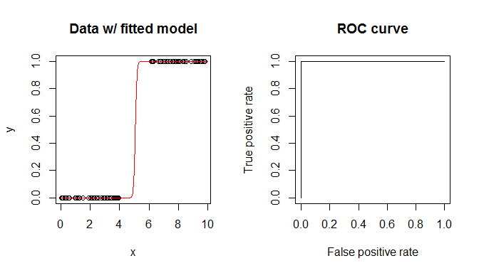
What you see in the output and in the figure is that the AUC is $1$. The AUC is the area under the ROC curve. The ROC curve is computed by varying the threshold above which you predict class $1$. At each point, you then examine the predicted classes vis-a-vie the actual classes and determine the true positive rate and the false positive rate. The ROC curve is just the plot of those two rates. Note however, that no matter what threshold you use, you will have perfect accuracy. Therefore, the ROC 'curve' is necessarily just the left and top sides of the unit square, and the area under it is $100\%$.
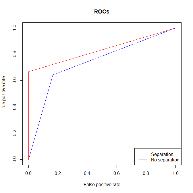
@Clif AB makes a good point that you can have separation without having an $AUC = 1$. Here is an illustration of that case. You can see that you nonetheless get a higher AUC when there is separation than an almost identical case without separation. The reason is essentially the same: no matter where you set your threshold, you will have a better true positive rate and false positive rate from the separable data than without.
x  = rep(0:1, each=10)
y1 = c(0,0,0,0,0,1,1,1,1,1,
       0,1,1,1,1,1,1,1,1,1)  # one 0 when x=1; no separation
y2 = c(0,0,0,0,0,1,1,1,1,1,
       1,1,1,1,1,1,1,1,1,1)  # no 0's when x=1; separation
m1 = glm(y1~x, family=binomial)
m2 = glm(y2~x, family=binomial)
summary(m1)  # output omitted
summary(m2)  # output omitted
pred1 = prediction(predict(m1, type="response"), y1)
perf1 = performance(pred1, "tpr", "fpr")
performance(pred1, "auc")@y.values[[1]]  # this is the AUC
# [1] 0.7380952
pred2 = prediction(predict(m2, type="response"), y2)
perf2 = performance(pred2, "tpr", "fpr")
performance(pred2, "auc")@y.values[[1]]  # this is the AUC
# [1] 0.8333333
windows()
  plot(perf1, col="blue", main="ROCs")
  plot(perf2, col="red", add=T)
  legend("bottomright", legend=c("Separation", "No separation"),
         lty=1, col=c("red","blue"))
-
4$\begingroup$ (+1) It's worth noting that one can have the issue of "perfect separation" without having AUC = 1. In particular, suppose that there was a dummy variable such that when $X_1 = 1$, it is always the case that $Y=1$...but when $X_1 = 0$, $Y$ can be either 0 or 1. Then $\hat \beta_1 = \infty$, but it is still possible that AUC < 1. $\endgroup$– Cliff ABCommented Dec 21, 2017 at 18:10
@gung had a great answer. I just want to add more explanations on why "no matter what threshold you use, you will have perfect accuracy"
If we add one more line to @gung's code to check the predicted probability, we can see this: essentially for all the data points the predicted probability ether 0 or 1, this is why the threshold does not matter and we got 1 on AUC.
> predict(m,data.frame(x=x), type="response")
           1            2            3            4            5            6            7            8            9           10           11           12           13           14
2.220446e-16 2.220446e-16 2.220446e-16 2.220446e-16 2.220446e-16 2.220446e-16 2.220446e-16 4.384945e-10 2.220446e-16 5.245702e-12 2.220446e-16 2.220446e-16 2.220446e-16 2.220446e-16
          15           16           17           18           19           20           21           22           23           24           25           26           27           28
2.220446e-16 2.220446e-16 2.220446e-16 4.719935e-11 2.220446e-16 2.220446e-16 2.220446e-16 2.220446e-16 2.220446e-16 2.669394e-13 2.220446e-16 1.365883e-10 2.220446e-16 6.992038e-13
          29           30           31           32           33           34           35           36           37           38           39           40           41           42
2.220446e-16 5.435395e-12 2.220446e-16 2.220446e-16 2.220446e-16 2.220446e-16 5.922012e-12 2.220446e-16 2.220446e-16 2.220446e-16 2.220446e-16 2.220446e-16 2.220446e-16 2.220446e-16
          43           44           45           46           47           48           49           50           51           52           53           54           55           56
2.220446e-16 2.220446e-16 2.912038e-12 2.220446e-16 2.220446e-16 1.258165e-11 2.220446e-16 2.220446e-16 1.000000e+00 1.000000e+00 1.000000e+00 1.000000e+00 1.000000e+00 1.000000e+00
          57           58           59           60           61           62           63           64           65           66           67           68           69           70
1.000000e+00 1.000000e+00 1.000000e+00 1.000000e+00 1.000000e+00 1.000000e+00 1.000000e+00 1.000000e+00 1.000000e+00 1.000000e+00 1.000000e+00 1.000000e+00 1.000000e+00 1.000000e+00
          71           72           73           74           75           76           77           78           79           80           81           82           83           84
1.000000e+00 1.000000e+00 1.000000e+00 1.000000e+00 1.000000e+00 1.000000e+00 1.000000e+00 1.000000e+00 1.000000e+00 1.000000e+00 1.000000e+00 1.000000e+00 1.000000e+00 1.000000e+00
          85           86           87           88           89           90           91           92           93           94           95           96           97           98
1.000000e+00 1.000000e+00 1.000000e+00 1.000000e+00 1.000000e+00 1.000000e+00 1.000000e+00 1.000000e+00 1.000000e+00 1.000000e+00 1.000000e+00 1.000000e+00 1.000000e+00 1.000000e+00
          99          100
1.000000e+00 1.000000e+00
In the output there are 100 probability predictions on 100 data points. The first 50 data point's probability is 0s and the second half are 1s. Among all these 100 numbers, there are 2 uniqe values 0 and 1. If we select any threshold between 0 and 1, we will always have the perfect cut, exact same label as ground truth.


