Can I assume (log-)normality for this sample?

Question

Here's a Q-Q plot for my sample (notice the logarithmic Y axis); $n = 1000$:

As pointed out by whuber, this indicates that the underlying distribution is left-skewed (the right tail is shorter).

Using shapiro.test (on the log-transformed data) in R, I get a test statistic of $W = 0.9718$ and a p-value of $5.172\cdot10^{-13}$, which means that we formally reject the null hypothesis $H_0 : \text{the sample is normal distributed}$ at the 95% confidence level.

My question is: Is this good enough in practice for further analysis assuming (log-)normality? In particular, I would like to calculate confidence intervals for the means of similar samples using the approximate method by Cox and Land (described in the paper: Zou, G. Y., cindy Yan Huo and Taleban, J. (2009). Simple confidence intervals for lognormal means and their differences with environmental applications. Environmetrics 20, 172–180):

ci <- function (x) {
        y <- log(x)
        n <- length(y)
        s2 <- var(y)
        m <- mean(y) + s2 / 2
        z <- qnorm(1 - 0.05 / 2) # 95%
        #z <- qnorm(1 - 0.10 / 2) # 90%
        d <- z * sqrt(s2 / n + s2 * s2 / (2 * (n - 1)))

        return(c(exp(m - d), exp(m + d)))
}

I've noticed that the confidence intervals tend to be centered around a point which is slightly above the actual sample mean. For example:

> mean(x)
[1] 82.3076
> y <- log(x)
> exp(mean(y) + var(y) / 2)
[1] 91.22831

I think these two values should be the same under $H_0$.

Answer 1

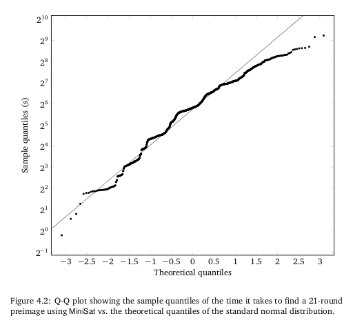
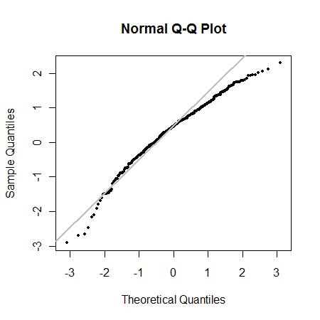
These data have a short tail compared to a lognormal distribution, not unlike a Gamma distribution:

set.seed(17)
par(mfcol=c(1,1))
x <- rgamma(500, 1.9)
qqnorm(log(x), pch=20, cex=.8, asp=1)
abline(mean(log(x)) + .1,1.2*sd(log(x)), col="Gray", lwd=2)

Nevertheless, because the data are strongly right-skewed, we can expect the largest values to play an important role in estimating the mean and its confidence interval. Therefore we should anticipate that a lognormal (LN) estimator will tend to overestimate the mean and the two confidence limits.

Let's check and, for comparison, use the usual estimators: that is, the sample mean and its normal-theory confidence interval. Note that the usual estimators rely only on the approximate normality of the sample mean, not of the data, and--with such a large dataset--can be expected to work well. To do this, we need a slight modification of the ci function:

ci <- function (x, alpha=.05) {
  z <- -qnorm(alpha / 2)
  y <- log(x); n <- length(y); s2 <- var(y)
  m <- mean(y) + s2 / 2
  d <- z * sqrt(s2 / n + s2 * s2 / (2 * (n - 1)))
  exp(c(mean=m, lcl=m-d, ucl=m+d))
}

Here is a parallel function for the normal-theory estimates:

ci.u <- function(x, alpha=.05) {
 mean(x) + sd(x) * c(mean=0, lcl=1, ucl=-1) / sqrt(length(x)) * qnorm(alpha/2)
}

Applied to this simulated dataset, the outputs are

> ci(x)
   mean     lcl     ucl 
2.03965 1.87712 2.21626 
> ci.u(x)
   mean     lcl     ucl 
1.94301 1.81382 2.07219 

The normal-theory estimates produced by ci.u look a little closer to the true mean of $1.9$, but it's hard to tell from one dataset which procedure tends to work better. To find out, let's simulate a lot of datasets:

trial <- function(n=500, k=1.9) {
  x <- rgamma(n, k)
  cbind(ci(x), ci.u(x))
}
set.seed(17)
sim <- replicate(5000, trial())

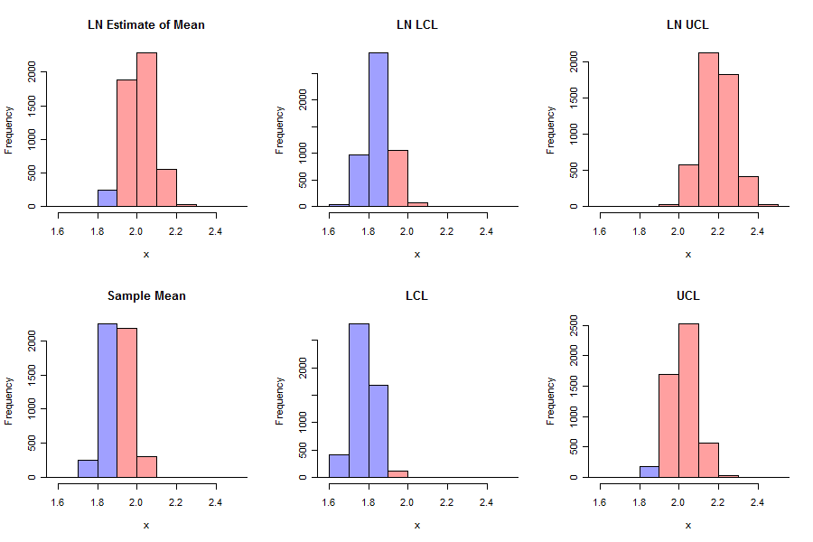
We are interested in comparing the outputs to the true mean of $1.9$. A panel of histograms is revealing in that regard:

xmin <- min(sim)
xmax <- max(sim)
h <- function(i, ...) {
  b <- seq(from=floor(xmin*10)/10, to=ceiling(xmax*10)/10, by=0.1)
  hist(sim[i,], freq=TRUE, breaks=b, col="#a0a0FF", xlab="x", xlim=c(xmin, xmax), ...)
  hist(sim[i,sim[i,] >= 1.9], add=TRUE,freq=TRUE, breaks=b, col="#FFa0a0",
                              xlab="x", xlim=c(xmin, xmax), ...)
}
par(mfcol=c(2,3))
h(1, main="LN Estimate of Mean")
h(4, main="Sample Mean")
h(2, main="LN LCL")
h(5, main="LCL")
h(3, main="LN UCL")
h(6, main="UCL")

It is now clear that the lognormal procedures tend to overestimate the mean and the confidence limits, whereas the usual procedures do a good job. We can estimate the coverages of the confidence interval procedures:

> sapply(c(LNLCL=2, LCL=5, LNUCL=3, UCL=6), function(i) sum(sim[i,] > 1.9)/dim(sim)[2])
 LNLCL    LCL  LNUCL    UCL 
0.2230 0.0234 1.0000 0.9648 

This calculation says:

• The LN lower limit will fail to cover the true mean about 22.3% of the time (instead of the intended 2.5%).

• The usual lower limit will fail to cover the true mean about 2.3% of the time, close to the intended 2.5%.

• The LN upper limit will always exceed the true mean (instead of falling below it 2.5% of the time as intended). This makes it a two-sided 100% - (22.3% + 0%) = 77.7% confidence interval instead of a 95% confidence interval.

• The usual upper limit will fail to cover the true mean about 100 - 96.5 = 3.5% of the time. This is a little greater than the intended value of 2.5%. The usual limits therefore comprise a two-sided 100% - (2.3% + 3.5%) = 94.2% confidence interval instead of a 95% confidence interval.

The reduction of the nominal coverage from 95% to 77.7% for the lognormal interval is terrible. The reduction to 94.2% for the usual interval is not bad at all and can be attributed to the effect of the skewness (of the raw data, not of their logarithms).

We have to conclude that further analyses of the mean should not assume lognormality.

Be careful! Some procedures (such as prediction limits) will be more sensitive to skewness than these confidence limits for the mean, so their skewed distribution may need to be accounted for. However, it looks unlikely that lognormal procedures will perform well with these data for practically any intended analysis.