Optimize likelihood function to get lambda for Box-Cox transform of two variables

Question

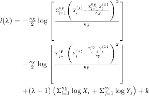
I'm trying to implement the Transformed Normal method (TN) that was described in Faraggi, D., & Reiser, B. (2002). Estimation of the area under the ROC curve. Statistics in medicine, 21(20), 3093–3106.

The authors transform the measurements of a diseased and a non-diseased sample to normality using a common $\hat{\lambda}$ in the Box-Cox-transformation and then proceed to calculate a cutpoint using normal theory.

The $\hat{\lambda}$ is obtained according to Zou, K. H., Tempany, C. M., Fielding, J. R., & Silverman, S. G. (1998). Original smooth receiver operating characteristic curve estimation from continuous data: Statistical methods for analyzing the predictive value of spiral CT of ureteral stones. Academic Radiology, 5(10), 680–687. https://doi.org/10.1016/S1076-6332(98)80562-X

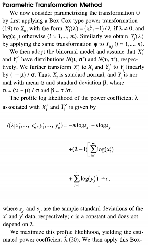
Here's the relevant part of the latter paper:

So a profile log likelihood function is constructed and optimized to find $\hat{\lambda}$. $x_{0,i}$ and $y_{0,j}$ are the original, unaltered measurements and $x'$ and $y'$ are the Box-Cox-transformed ones, if I understand the paper correctly.

I am now trying to implement this likelihood function in R. Apparently, the Box-Cox-transformed variables are inserted into the likelihood function, so my attempt looks like this:

boxcox <- function(x, lambda) {
    if (lambda == 0) {
        return(log(x))
    } else {
        ((x**lambda) - 1) / lambda
    }
}

profile_loglik <- function(lambda, x, y) {
    m <- length(x)
    n <- length(y)
    x_t <- boxcox(x, lambda)
    y_t <- boxcox(y, lambda)
    return(-m * log(sd(x_t)) - n * log(sd(y_t)) + (lambda - 1) * (sum(log(x_t)) + sum(log(y_t))))
}

calc_lambda_hat <- function(x, y) {
    optim_func <- function(lambda) -(profile_loglik(lambda = lambda, x = x, y = y))
    optim(0.5, optim_func, method = "Brent", lower = 0, upper = 100)
}

# Example data
x <- rlnorm(200)
y <- rlnorm(100, 0.4, 0.4)
calc_lambda_hat(x, y)

# Result:
$par
[1] 100

$value
[1] NaN

$counts
function gradient 
      NA       NA 

$convergence
[1] 0

$message
NULL

# Plus lots of warnings...

The data of Zou et al. seem to be roughly lognormally distributed and so is the data I have in mind, so the method should be applicable. However, since some of the $x'$ and $y'$ will become negative after the Box-Cox transformation, terms like $log(x')$ in the likelihood function become NaN. If I insert $x_0$ and $y_0$ instead of $x'$ and $y'$ into the likelihood function, it is a monotonically increasing function.

Thus, my question is: What are the mistakes in my implementation? Thank you.

Answer 1

Bantis, L. E., Nakas, C. T. and Reiser, B. (2014), Construction of confidence regions in the ROC space after the estimation of the optimal Youden index‐based cut‐off point. Biom, 70: 212-223. doi:10.1111/biom.12107 implements the method and gives the following formula:

We see that they use the transformed values when calculating the standard deviations (in the square brackets) but the untransformed values in the third row of the formula.

Again, I implemented this in R and this time my only quibble is that $-\frac{n_X}{2}$ and $-\frac{n_Y}{2}$ apparently should be replaced by just $-n_X$ and $-n_Y$, which are in my understanding the numbers of observations in both groups, otherwise the results are way off. The R code thus is:

profile_loglik <- function(lambda, x, y) {
    m <- length(x)
    n <- length(y)
    x_t <- boxcox(x, lambda)
    y_t <- boxcox(y, lambda)
    -m * log(sd(x_t)) - n * log(sd(y_t)) + (lambda - 1) * (sum(log(x)) + sum(log(y)))
}

calc_lambda_hat <- function(x, y) {
    optim_func <- function(lambda) -(profile_loglik(lambda = lambda, x = x, y = y))
    optim(0.5, optim_func, method = "L-BFGS-B", lower = -4, upper = 10)
}

I tested calc_lambda_hat against concatenating both groups and then using forecast::BoxCox.lambda(c(x, y), "loglik"). The correlation of the returned values for $\lambda$ after 1000 repetitions in various scenarios with lognormal distributions is about 85%, so this way the implementation seems to be OK.