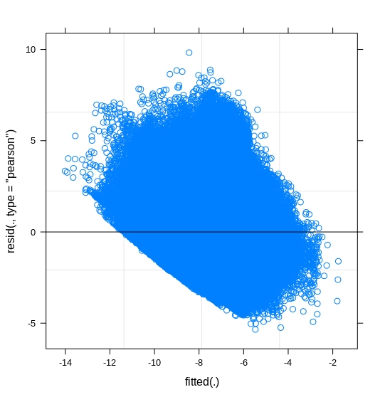
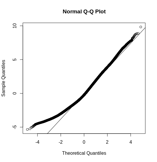
What do these two plots mean? Does the same set of assumptions (normality of residuals; homogenity of variance) apply for linear mixed effects model? Am I right in reading that this model is not properly specified as it violates normality assumptions?
The residual plots reflect that the assumptions of residual normality and homogeneity are violated. This affects inference but not point estimates of the model: The p-value and confidence intervals of each coefficient, as well as confidence and prediction intervals of predicted means, are doubtful. The point estimates of fixed effects' coefficients and predicted random effects are still unbiased. This is because the standard errors of each fixed-effect coefficient is biased, despite its consistency if the number of groups (country and sector in your case) and the number of customers clustered in each group are large https://thestatsgeek.com/2014/08/17/robustness-of-linear-mixed-models/.
In addition to a limited range of the dependent variable, these violations can be caused by other peculiarity, such as the functional form of predictors. You should make a plot between each response-predictor pair to help determine the function form. Try at least logarithm, quadratic and cubic terms of loan amount and interaction terms between gender and loan amount to remove part of the nonnormality and heterogeneity in the error term. Coefficients in a fixed-effect specification in the form of log(y) ~ log(x) measures elasticity directly. Add additional predictors may substantially improve the residual diagnosis results. Check the fixed-effect predictor significance by anova() with estimation by ML.
The clustering structure also needs attention, as I don't think that Sector S in Country A is comparable with Sector S in Country B to share the same random effects of sector. Perhaps clustering by country-specific sector alone is better, which requires coding each country-sector pair as a unique group. Further, variables with random effects also need investigation. The intercept has random effects in your current model specification. However, this within-country and within-sector variability might differ by gender. And there might be a random slope if the effect of loan amount on time to loan deviates by country-sector pair, and this random slope might be correlated with the random intercept. Therefore, a tentative random effect specification might be (0 + borrower.Gender + log(borrowing.Amount) | interaction(borrower.Country, borrower.Sector)), where 0 + borrower.Gender moves random intercepts to around the gender indicator, so the standard deviation of random intercepts differ by gender. You can compare this random-effect specification with your current crossed clustering by a likelihood ratio test, using anova() with estimation by REML, varCompTest() in {varTestnlme}, exactRLRT() in {RLRsim}, and PBmodcomp() in {pbkrtest}.
If your purpose is to make predictions, then there is no need to correct for the assumption violations, as the coefficient point estimates are unbiased. If you need to conduct hypothesis testing, determine predictor significance, and build confidence intervals, then consider modeling heterogeneity with lme(weights =) in Package {nlme} and using cluster-robust standard errors through vcovCR() in {clubSandwich}. As your sample size is huge in terms of the numbers of customers, countries, and sectors, the difference in standard errors between a standard linear mixed model and heterogeneity-corrected, cluster-robust results might be minimal.
My dataset consists of only those that have received loans. So I assume right censoring does not apply for Time.to.obtain.loan.
If you intend to make any causal inference, such as whether gender and requested amount affect loan processing time, using data of only loan receivers constitutes a sample-selection bias. Instead, you should use data of all loan requesters although the processing time might be only observable on loan receivers. Check package {sampleSelection}. See Toomet, O., & Henningsen, A. (2008). Sample selection models in R: Package sampleSelection. Journal of Statistical Software, 27(7). https://doi.org/10.18637/jss.v027.i07 and Bushway, S., Johnson, B. D., & Slocum, L. A. (2007). Is the magic still there? The use of the Heckman two-step correction for selection bias in criminology. Journal of Quantitative Criminology, 23(2), 151–178. https://doi.org/10.1007/s10940-007-9024-4
If you are instead interested in observational relationship, using records of loan receivers alone is fine. I agree with Dimitris Rizopoulos that the data structure calls for survival analysis, as the dependent variable is a duration. Ideally, you should acquire data of those still under processing, so the time to obtain loans is not completely finished observing and involves right censoring. Even if the data do not exhibit right censoring, using survival analysis is still a good choice. However, survival analysis has its own assumptions, such as proportional hazards in a Cox model coxph(). Package {coxme} may not be necessary, as the regular Package {survival} can deal with clustered errors through coxph(..., cluster()) and random intercepts through coxph(..., frailty()), but I think it could handle only one level of clustering. See an example of mixed-effect Cox regression from UCLA https://stats.oarc.ucla.edu/r/dae/mixed-effects-cox-regression/
Do you perhaps have (many) zeros in the Time.to.obtain.loan? If this is the case, indeed assuming a normal distribution would not be optimal. You could give a try to a Beta mixed effects models.
Beta regression is for proportional response, where the dependent variable is a fraction between zero and one, and there is zero- and one-inflated beta regression. The data structure does not appear to align with that assumed by beta regression. Instead, if the response is positive, gamma regression can be used. The result might be very similar to a linear regression with logarithm-transformed response. See a tutorial of gamma regression with shape and scale parameters' meaning and calculation explained https://data.library.virginia.edu/getting-started-with-gamma-regression/. Still, the best option for a duration response is survival analysis.
although the Time.to.obtain.loan is not a count variable, can one use poisson model from GLMMAdaptive?
Yes, you may need special packages to achieve it, as the regular Poisson regression model in glm(family = poisson) allows only integers in the dependent variable. You can of course round the time to obtain loans to make it integer. Package {glmmTMB} worked best for me so far in count data modeling. It allows a noninteger dependent variable, zero inflation, dispersion effects, and random effects for repeated measurements and clustered errors. You could use clustered standard errors for glmmTMB() models though, perhaps through vcovHC() in {sandwich} and vcovCR() in {clubSandwich}. Again, the best option for a duration response should be survival analysis.


