How to model data in jags/bugs generated by taking the minimum of two random variables?

Question

I have been thinking of modeling human timing data using jags where the data comes from an experiment where participants tap in time with a very slow metronome. The data is then a number of measurements of how "off" the tap was compared to the metronome. The data could be thought of as coming from a normal distribution. This would then be mock-up data for 10000 taps (using R):

timing_distribution <- rnorm(10000, 0, 300)

The problem is that when participants overshoot the target interval they instead react to the metronome tone. Say that reaction time is also from a normal distribution then mock-up data would be:

reaction_time_distribution <- rnorm(10000, 250, 50)

The timing distribution and the reaction time distribution could then be though of as being combined into a joint distribution like this:

joint_distribution <- pmin(timing_distribution, reaction_time_distribution)

That is whatever comes first the timing impulse or the reaction to tap after the metronome tone results in a tap.

My question is how could one go about modeling this in jags/bugs? What I'm after is someth ing like this

model {
    for( i in 1 : N ) {
 y[i] ~ min( dnorm( muTiming , tauTiming ), dnorm( muReaction , tauReaction ))
}
tauTiming ~ dgamma( 0.01 , 0.01 )
muTiming ~ dnorm( 0 , 1.0E-10 )
tauReaction ~ dgamma( 0.01 , 0.01 )
muReaction ~ dnorm( 0 , 1.0E-10 )

}

But I guess that y[i] ~ min( dnorm( muTiming , tauTiming ), dnorm( muReaction , tauReaction )) is not really possible in jags...

Answer 1

What seems to work, and what I ended up doing, was to define a new sampling distribution using the "ones trick" described in the BUGS manual and with and example for jags given here.

For the "ones" trick to work I need to define the likelihood function for my new distribution, which is the same as the [probability density function] but with the data as the variable argument instead of the parameters.

Using the following equality, where $X$ and $Y$ are random variables and $x$ is a constant:

$ prob(min(X, Y)>x) = prob(X>x\ and\ Y>x) = prob(X>x) \cdot prob(Y>x) $

I can construct the cumulative density function for my special distribution as follows:

$ prob(min(norm1, norm2) < x) \Rightarrow 1 - prob(min(norm1, norm2) > x) \Rightarrow 1 - prob(norm1 > x\ and\ norm2 > x) \Rightarrow 1 - prob(norm1>x) \cdot prob(norm2>x) \Rightarrow 1 - (1 - prob(norm1<x)) \cdot (1 - prob(norm2<x))$

As $prob(norm1 < z)$ is the cumulative density function of a normal distribution the final "special" cumulative density function is:

$1 - (1 - pnorm(x,\mu_1, \sigma_1)) \cdot (1-pnorm(x,\mu_2, \sigma_2))$

To get the probability density function I differentiate this using the product rule:

$ h(x)=f_1(x)*f_2(x) \Rightarrow h'(x) = f_2'(x)*f_1(x) + f_1'(x)*f_2(x)$

and end up with the following R expression:

-(-dnorm(x, m1, s1) * (1 - pnorm(x, m2, s2)) + -dnorm(x, m2, s2) * (1 - pnorm(x, m1, s1)))

In jags the final model specification became (notice that s1 has become 1/pow(s1, 2) due to jags using precision instead of SD):

model{
    for (i in 1:n){
    p[i] <- -(-dnorm(x[i], m1, 1/pow(s1, 2)) * (1 - pnorm(x[i], m2, 1/pow(s2, 2))) + -dnorm(x[i], m2, 1/pow(s2, 2)) * (1 - pnorm(x[i], m1, 1/pow(s1, 2))))
    ones[i] ~ dbern(p[i])
    }
    m1_sd <- 1000
    m1 ~ dnorm(0, 1/pow(m1_sd, 2))
    m2_sd <- 1000
    m2 ~ dnorm(400, 1/pow(m2_sd, 2))
    s1_m <- 400 
    s1_s <- 1000
    s1 ~ dgamma(pow(s1_m,2)/pow(s1_s,2), s1_m/pow(s1_s,2))
    s2_m <- 100 
    s2_s <- 1000
    s2 ~ dgamma(pow(s2_m,2)/pow(s2_s,2), s2_m/pow(s2_s,2))
}

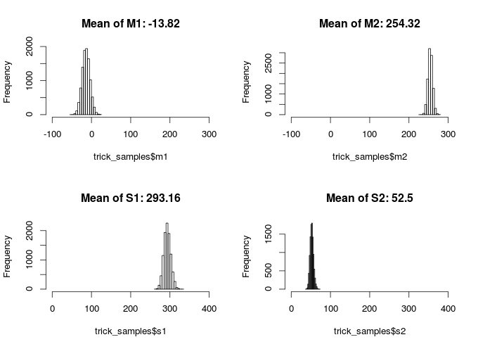
This model seems to (and should) retrieve the original parameters as the following 10000 sample posteriors show:

Answer 2

I'm sure more informed people will help you here more than I can. But here's a quick suggestion. Shouldn't you model the data in a different way? I was thinking of something like this:

y[i] ~ pi1*N(mu1, sigma1) + pi2*N(mu2, sigma2)

where pi1 + pi2 = 0 and you can think of pi1 and pi2 as parameters of a latent indicator variable that says which group each observation belongs to.

Then you can look at some examples from Bugs about mixture models and see if it works. See this example.