Fitting a partial distribution to a normal distribution

Question

So, I've got a(n assumed) normal distribution that is left bound by 0, and I'm trying to extrapolate what would happen if the distribution could go negative.

Given a portion of the right tail of a normal distribution, is there a good method for building out the rest of the distribution?

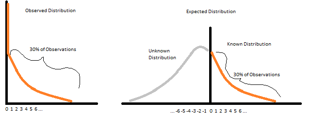
For instance, in the below image, taking the observations at 0 and estimating the grey unknown distribution:

Edit:

To clarify, in most cases we'll know the second and third standard deviations (inferred from the percent of observations on the right side of the curve) from the mean, but not the mean itself - and, we want to find the mean an plot the unknown distribution (grey in the above picture).

Admittedly, I'm rusty in this area, so forgive me if this is a poor question.

Would it make sense to take the distance between the far right 2.1% of observations, call that the standard deviation and infer the mean and variance form that?

Answer 1

This is called a zero-censored normal distribution. The likelihood function is

P(Y<0 | mu,sigma) for y = 0, and p(Y=y | mu,sigma) for y > 0

You can find the ML estimator using this R code:
y = rnorm(10000,0.5,2) # simulate some sample data 
y[y<0]=0 # censor at zero
minlogL = function (p ) { 
  mu = p[1]
  logsigma=p[2] # must used log-sigma because the second parameter can be negative while sigma must be positive
  return(sum(-log(dnorm(y[y>0],mu,exp(logsigma)))) - sum(y<=0)*log(pnorm(0,mu,exp(logsigma))))
}
nlm(minlogL,c(0,0)) 

Answer 2

@Helene Hoegsbro Thygesen has the right answer ... I missed that the lower truncation was given and that the observations at 0 were given.

Since I wrote it anyway I post the script for estimating mean and variance

(1) without knowing the lower truncation point

(2) without point probability at zero

the likelihood is then based on the truncated normal density

$$ f(x|\mu,\sigma,\xi) = \frac{1}{1-\Phi\left(\xi\right)} * \frac{1}{\sigma} \phi\left(\frac{x-\mu}{\sigma}\right)$$

The script runs estimation on 1000 samples and plots distribution of estimator

library(Rsolnp)
M <- matrix(0,ncol=4,nrow=1000)
for (i in 1:1000)
{
    N <- 3000
    x <- rnorm(N,sd=2)-1
    x <- x[which(x>0)]
    x_hat <- min(x)

loglik<-function(theta)
    {
        a <- theta[1]
        b <- exp(theta[2])
        denom <- 1 - pnorm(x_hat,mean=a,sd=sqrt(b))
        ll <- sum( log( dnorm(x,mean=a,sd=sqrt(b))/denom))
        return(-ll)
    }


model <- solnp(c(0,2),loglik,LB=c(-5,-5),UB=c(5,5))
# variance estimate
M[i,1]<-exp(model$pars[2])
# mean estimate
M[i,2]<-model$pars[1]
M[i,3]<-length(x)
M[i,4]<-model$convergence
print(i)
flush.console()
}

layout(matrix(c(1,2,3),ncol=3))
hist(M[,1])
hist(M[,2])
hist(M[,3])
table(M[,4])