I have an insignificant beta weight of a predictor, which the only predictor in a step with significant R-square change and significant F-value

Question

I am running a hierarchichal multiple linear regression with 4 steps containing theoretically justifyable variables:

Outcome: pain rating Step 1: demographic variables (age, gender) Step 2: Pain sensitivity measures (2 variables) Step 3: cognitive function (1 variable) Step 4: specific thoughts regarding pain (2 variables)

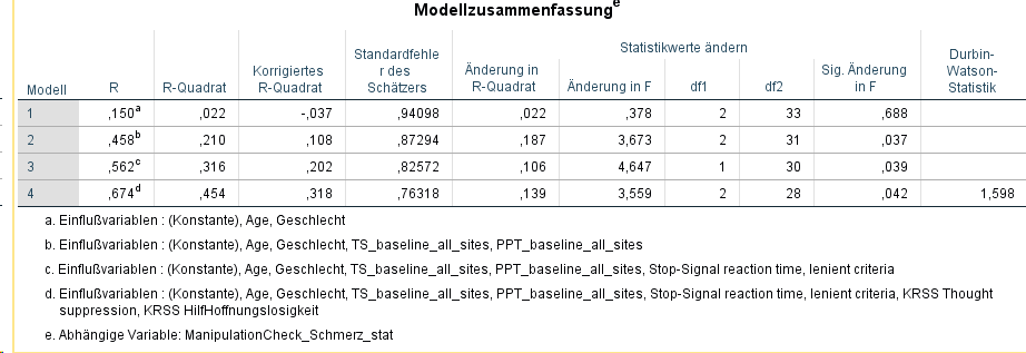
Here is my problem: when entering the cognitive function variable (calles Stop-Signal reaction time, lenient criteria) in Step 4, the change in R square is significant

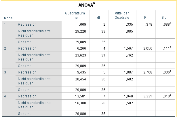
Also the F-Test is significant:

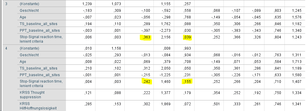
However, in the final model, the standardized beta (first yellow column) of the Step 3 variable is not significant (second yellow column). This seems to be only the case after the variables of step 4 have been entered:

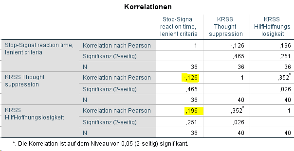
The variables of Step 4 are not correlated with the variable in Step 3:

Thus, it doesn't seem to be a problem of multicollinearity. I cannot make sense of this and I appreciate any help!

---

Thank you very much for your helpful suggestions!

Indeed, there are some interesting effects when looking at KRSS thought suppression and KRSS hilf/Hoffnungslosigkeit. For the sake of clarity, I will only report the results regarding KRSS thought suppression now.

It actually seems that Stop-Signal RT is not affected by thought suppression, as the beta weight nearly stays the same and is still significant. However, PPT_baseline (PPT_prestat_all_sites in this table) is nearly half after introducing thought suppression:

Indeed, there is a significant inverse correlation between thought suppression and PPT baseline (r= -.39, p=.012) which also makes sense in light of the theoretical background.

Would it be suitable to do a moderation analysis at this point, with baseline PPT as a moderator for the relationship between thought suppression and the outcome variable exercise-induced pain? Theoretically, that would make sense. However, the sample size appears to be too small to do that (N=40), and, as the coefficient table shows baseline PPT and the outcome are not correlated.

Thank you!

Answer 1

When moving from model 3 to 4, you are adding two variables instead of one. Not only are you adding $g + h$ but implicitly the interaction $g * h$. If there is no evidence of a correlation, there could potentially be an interaction effect between the two KRSS measures that moderates (i.e. attenuates) the effect of the Stop-Signal RT $(0.242 < 0.363)$ as well as the PPT baseline $(-0.397 < -0.215)$.

However, I would first isolate each of the KRSS measures and build two models, let's call them 4a and 4b. In 4a you add the KRSS Thought suppresion measure to Model 3, and in 4b you instead add KRSS HilfHoffnungslosigkeit. These two steps could rule out any individual moderation and validate your correlation analysis.

In case neither the models 4a or 4b individually moderate the RT or the PPT scores, it is likely a moderation-by-interaction effect.

To test this for the interaction $g * h$, compute a new variable: KRSS Thought Suppresion * KRSS HilfHoffnungslosigkeit and include this variable in the correlation analysis. (If the variables are of different scales, you should standardize them before the multiplication.)

Also note that gender seems to play a much lesser role in Model 4 than in 3: $(-0.1 << -0.013)$, suggesting perhaps that this effect was absorbed by one of the KRSS variables.

If you are interested in the effects of adding variables, a more detailed approach would be to extend the analysis with mediation^[1] / moderation^[2] analysis. That is also the basis for my recommendation, so the procedure is similar, but if you have a grasp of these concepts you can make a nice flow chart.

Finally, because the $F$-test for models 1 and 2 are not significant, you could exclude these variables from the final model. Naturally, you should still report the negative findings of the hierarchical analysis. You could also plot each model in a single plot and compare the slopes and the intercepts to get a sense of how the hierarchical steps affect the model. If you are using SPSS, use the Save function in the Regression window and then create a combined line plot of the $\hat y$ values for each model.

I hope this helps.

Answer 2

In addition to noumenal's explanation, I would point out that by adding a new variable, you are also changing the coefficients for existing variables, as they now control for your new addition. It seems plausible to me that you could add a new variable that improves the fit of other variables to the outcome (by accounting for confounding variance that was previously just error) without the new variable itself contributing significantly to the outcome. In other words - your results make sense to me, and I don't think it would be necessary for the new variable to be statistically significant for the model to be improved.