What is allowable deviation from desired significance/coverage?

Question

Consider performing a statistical hypothesis test and wants to achieve significance $\alpha$. What is a good rule of thumb for an allowable deviation from the desired confidence level?

Say I want to perform a hypothesis test with $\alpha=0.05$, but given the actual nature of the underlying processes and test applied, the true probability of type I error is $0.01$ or $0.10$, is this generally acceptable? Surely there are at least a few widely agreed upon standards for what decision from desired $\alpha$ is acceptable.

As an example, I've been investigating one-way ANOVA, to test the interaction of unequal variance, non-normality, and unequal sample sizes on the actual probability of rejecting the hypothesis of equal means. As long as the population variances are within a factor of even 10 of each other (for normal, factor of 4 seems good even for exponential) then it does seem to give significance close to the desired level. I also find that the populations with large variance having the same or larger sample size (but not like an order of magnitude larger) as compared to the populations with smaller variance, then it is also fairly robust still. The true probability of type I error is usually from $1\%$ to $10\%$ when actually shooting for a $5\%$ level, if these factors are controlled reasonably.

My gut tells me that a deviation of $\pm 3\%$ or so from a desired level of $5\%$ would be acceptable.

So the question is: what deviation from $\alpha$ is generally acceptable for hypothesis tests?

Here is my (probably very inefficient) R code for investigating 1-way anova with deviations from normality and equal variances:

NS=10000
sstrd=vector("numeric",length=NS)
ssed=sstrd
sstd=sstrd
nv=round(c(5+runif(1)*10,
           5+runif(1)*10,
           5+runif(1)*10,
           5+runif(1)*10))
mv=c(0,0,0,0)
sv=c(1,1+runif(1)*1.5,1+runif(1)*2,1+runif(1)*3)
for (ns in 1:NS){
  x1=rnorm(nv[1],mv[1],sv[1]) #rexp(nv[1],1/sv[1])-sv[1] #
  x2=rnorm(nv[2],mv[2],sv[2]) #rexp(nv[2],1/sv[2])-sv[2]
  x3=rnorm(nv[3],mv[3],sv[3]) #rexp(nv[3],1/sv[3])-sv[3]
  x4=rnorm(nv[4],mv[4],sv[4]) #rexp(nv[4],1/sv[4])-sv[4]
  data=c(x1,x2,x3,x4)
  group=c(rep("A1",length(x1)),rep("A2",length(x2)),rep("A3",length(x3)),rep("A4",length(x4)))
  group=as.factor(group)
  xdd=mean(data)
  SST=sum((data-xdd)^2)
  g=levels(group)
  k=length(g)
  n=length(data)
  nvec=as.numeric(table(group))
  SSTr=0
  xd=vector("numeric",length=length(g))
  for (i in 1:length(g)){
    xd[i]=mean(data[group==g[i]])
    SSTr=SSTr+nvec[i]*(xd[i]-xdd)^2
  }
  xdvec=NULL
  for (i in 1:length(g)){
    xdvec=c(xdvec,rep(xd[i],nvec[i]))
  }
  SSE=sum((data-xdvec)^2)
  pv=nv/sum(nv)
  spvm=c(sum(pv[c(2,3,4)]),sum(pv[c(1,3,4)]),sum(pv[c(1,2,4)]),sum(pv[c(1,2,3)]))
  sta=sum(sv^2*((1-pv)^2+pv*spvm))
  sstrd[ns]=SSTr
  sstd[ns]=SST
  ssed[ns]=SSE
}
sta
c(mean(sstd),sd(sstd))
c(mean(sstrd),sd(sstrd))
c(mean(ssed),sd(ssed))
f=(sstrd/3)/(ssed/(sum(nv)-4))
plot(ecdf(f))
xv=seq(0,max(f),length=1000)
lines(xv,pf(xv,3,sum(nv)-4),col="red")
1-sum(f<=qf(0.95,3,sum(nv)-4))/length(f) # actual 1-alpha

Assuming a desired level of $\alpha=5\%$, the last line of code is where I calculate the actual probability of going beyond the threshold $f$ value.

I'm not looking for corrections to my R code, per se, but feel free to point out any errors if there are any.

Answer 1

I think this kind of exploration of the robustness of one-factor ANOVA is very worthwhile. There are several reasons you might not have found interesting results. Let me explore in the direction of my top two best guesses: (a) You might not be looking at the deviations from assumption that cause real problems. (b) Your code may not be doing exactly what you expect.

Regarding (a): It is well known that the pooled two-sample t test fails when sample sizes differ and the smaller sample has the greater population variance. In particular, the true level of significance may be much larger than the intended 5% level. The Welch t test handles this situation much better.

Because the traditional one-factor ANOVA is a generalization of the pooled t test to accommodate $k > 2$ levels of the factor, it is reasonable to expect that the ANOVA will behave badly for an unbalanced design in which the smallest number of replications matches the level with the greatest population variance. So let's start by looking there.

Regarding (b): At least at the start, it is best to use built-in functions to use pre-debugged code. Then when everything is working as it should, maybe try to substitute your own code to speed up the simulation.

For example, here is R code for getting the P-value of a particular ANOVA.

# Generate random data to specifications
set.seed(2019)
x1 = rnorm(5, 100, 10)  # note small nr of reps
x2 = rnorm(10, 100, 10)
x3 = rnorm(10, 100, 10)
x = c(x1,x2,x3)
g = as.factor(rep(1:3, c(5,10,10)))
# 'Steal' P-value from built-in function
anova(lm(x ~ g))
Analysis of Variance Table

Response: x
          Df  Sum Sq Mean Sq F value Pr(>F)
g          2   37.53  18.767  0.1547 0.8576  # <-- P-value here
Residuals 22 2668.23 121.283  
anova(lm(x ~ g))[1,5]                        # Pick it off
[1] 0.8575656

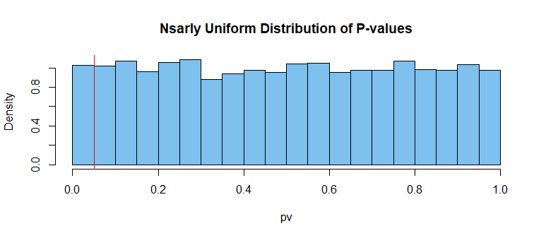
All assumptions of ANOVA are met, $H_0$ is true, and P-value exceeds 5%, as expected (most of the time).

Assumptions met: Now let's replicate the above m = 10^4 times and check that the true significance level is 5%.

set.seed(2019)
m = 10^4;  pv=numeric(m)   # wrap above code in a for-loop
for(i in 1:m) {
  x1=rnorm(5,100,10); x2=rnorm(10,100,10); x3=rnorm(10,100,10)
  x = c(x1,x2,x3); g = as.factor(rep(1:3, c(5,10,10)))
  pv[i]=anova(lm(x~g))[1,5] }
mean(pv<=.05)
[1] 0.0512
2*sd(pv<=.05)/sqrt(m)   # aprx 95% margin of simulation error
[1] 0.004408329

The rejection rate is close to 5% $(0.05 \pm 0.004).$ Using m=10^6 iterations would give almost exactly 5%, but that would require a faster computer or more patience than I have right now.

Also, the distribution of the P-values is very nearly uniform, as one expects when $H_0$ is true and assumptions are met.

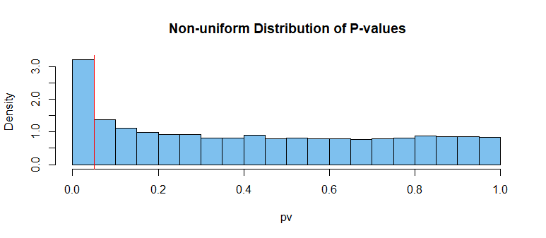
Unbalanced, heteroscedastic: Finally, lets try looking at the result when variances are unequal, as described earlier with $n_1 = 5; \sigma_1 = 25:$

set.seed(629)
m = 10^4;  pv=numeric(m)
for(i in 1:m) {
 x1 = rnorm(5,100,25); x2 = rnorm(10,100,10); x3 = rnorm(10,100,10)
 x = c(x1,x2,x3); g = as.factor(rep(1:3, c(5,10,10)))
 pv[i]=anova(lm(x~g))[1,5] }
mean(pv<=.05)
[1] 0.1602
2*sd(pv<=.05)/sqrt(m)
[1] 0.007336196

Now, the true significance level is about 16% $(0.160 \pm 0.007).$

For this simulation, the distribution of the P-values is clearly not uniformly distributed. Because $H_0$ is true, this is an indication that assumptions are not met.

Notes: The method of 'stealing' P-values from built-in functions runs relatively slowly. I guess the main reason is that R takes the trouble to format the entire ANOVA table, from which I pick off only the P-value.

If you're doing a lot of these simulations, it's worthwhile writing your own code. But make sure it gives the same P-value as the built-in R procedure. Starting with the same seed, you should get the same answer.

You can check power against various alternatives using essentially the same code. Perhaps compare results with true and false $H_0$'s using anova(lm) and the Welch version of the one-factor ANOVA using oneway.test.

If you're exploring effects of non-normal data I think it may be fruitful to explore exponential data with small numbers of replications. (Poisson data is also heteroscedastic, if $H_0$ is false, but I have not found interesting difficulties with Poisson data. To the point of wondering if the square-root transformation is worthwhile in a one-factor ANOVA.)