Estimating the probability that a software change fixed a problem

Question

At work we have a hardware device that is failing for some yet to be determined reason. I have been tasked to see if I can make this device not fail by making changes to its software driver. I have constructed a software test bench which iterates over the driver functions which I feel are most likely to cause the device to fail. So far I have forced 7 such failures and the iterations that the device failed on are as follows:

100 22 36 44 89 24 74

Mean = 55.57 Stdev = 31.81

Next, I made some software changes to the device driver and was able to run the device for 223 iterations without failure before I manually stopped the test.

I want to be able to go back to my boss and say "The fact that we were able to run the device for 223 iterations without failure means that my software change has a X% probability of fixing the problem." I would also be satisfied with the converse probability that the device will still fail with this fix.

If we were to assume that the iteration the device fails on is normally distributed, we can say that going 223 iterations without failure is 5.26 standard deviations from the mean which roughly has a 1-in-14 million chance of happening. However, because we only have a sample size of 7 (not including the 223), I'm fairly certain it would be unwise to assume normality.

This is where I think the Student's t-test comes into play. Using the t-test with 6 degrees of freedom, I've calculated that the actual population mean has a 99% probability of being less than 94.

So now my question to you guys is whether or not I am allowed to say with 99% certainty that hitting 223 iterations without failure is a 4.05 sigma event, i.e. $\frac{(223 - 94)}{31.81} = 4.05$ ? Am I allowed to use the 31.81 sample standard deviation in that calculation or is there some other test I should do to get a 99% confidence on what the maximum standard deviation is and then use that in my calculation for how many sigmas 223 really is away from the mean at the 99% confidence level?

Thanks!

UPDATE

The answers I received here are beyond any expectation I had. I truly appreciate the time and thought many of you have put into your answers. There is much for me to think about.

In response to whuber's concern that the data does not seem to follow an exponential distribution, I believe I have the answer for as to why. Some of these trials were run with what I thought would be a software fix but ultimately ended in failure. I would not be surprised if those trials were the 74 89 100 grouping that we see. Although I wasn't able to fix the problem it certainly seems like I was able to skew the data. I will check my notes to see if this is the case and my apologies for not remembering to include that piece of information earlier.

Lets assume the above is true and we were to remove 74 89 100 from the data set. If I were to re-run the device with the original driver and get additional failure data points with values 15 20 23, how would you then compute the exponentially distributed parametric prediction limit at the 95% confidence level? Would you feel that this prediction limit is still a better statistic than assuming independent Bernoulli trials to find the probability of no failure at 223 iterations?

Looking more closely at the wikipedia page on Prediction Limits I calculated the parametric prediction limits at the 99% confidence level assuming unknown population mean and unknown stdev on Excel as follows:

$\bar{X_n} = 55.57$
$S_n = 31.81$
$T_a = T.INV\Bigl(\frac{1+.99}{2},6\Bigr)$

$Lower Limit = 55.57 - 3.707*31.81*\sqrt{1+\frac{1}{7}} = -70.51$
$Upper Limit = 55.57 + 3.707*31.81*\sqrt{1+\frac{1}{7}} = 181.65$

Since my trial of 223 is outside the 99% confidence interval of [-70.51 , 181.65] can I assume with 99% probability that this is fixed assuming that the underlying distribution is the T-Distribution? I wanted to make sure my understanding was correct even though the underlying distribution is most likely exponential, not normal. I have no clue in the slightest how to adjust the equation for an underlying exponential distribution.

UPDATE 2

So I'm really intrigued with this 'R' software, I've never seen it before. Back when I took my stats class (several years ago) we used SAS. Anyway, with the cursory knowledge I gathered from Owe Jessen's example and a bit of help from Google, I think I came up with the following R code to produce the Prediction Limits with the hypothetical dataset assuming an Exponential Distribution

Let me know if I got this right:

fails <- c(22, 24, 36, 44, 15, 20, 23)
fails_xfm <- fails^(1/3)
Y_bar <- mean(fails_xfm)
Sy <- sd(fails_xfm)
df <- length(fails_xfm) - 1
no_fail <- 223

percentile <- c(.9000, .9500, .9750, .9900, .9950, .9990, .9995, .9999)
quantile <- qt(percentile, df)

UPL <- (Y_bar + quantile*Sy*sqrt(1+(1/length(fails_xfm))))^3
plot(percentile,UPL)
abline(h=no_fail,col="red") 
text(percentile, UPL, percentile, cex=0.9, pos=2, col="red")

Prediction Limits http://img411.imageshack.us/img411/5246/grafr.png

Answer 1

This question asks for a prediction limit. This tests whether a future statistic is "consistent" with previous data. (In this case, the future statistic is the post-fix value of 223.) It accounts for a chance mechanism or uncertainty in three ways:

1. The data themselves can vary by chance.

2. Because of this, any estimates made from the data are uncertain.

3. The future statistic can also vary by chance.

Estimating a probability distribution from the data handles (1). But if you simply compare the future value to predictions from that distribution you are ignoring (2) and (3). This will exaggerate the significance of any difference that you note. This is why it can be important to use a prediction limit method rather than some ad hoc method.

Failure times are often taken to be exponentially distributed (which is essentially a continuous version of a geometric distribution). The exponential is a special case of the Gamma distribution with "shape parameter" 1. Approximate prediction limit methods for gamma distributions have been worked out, as published by Krishnamoorthy, Mathew, and Mukherjee in a 2008 Technometrics article. The calculations are relatively simple. I won't discuss them here because there are more important issues to attend to first.

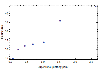
Before applying any parametric procedure you should check that the data at least approximately conform to the procedure's assumptions. In this case we can check whether the data look exponential (or geometric) by making an exponential probability plot. This procedure matches the sorted data values $k_1, k_2, \ldots, k_7$ = $22, 24, 36, 44, 74, 89, 100$ to percentage points of (any) exponential distribution, which can be computed as the negative logarithms of $1 - (1 - 1/2)/7, 1 - (2 - 1/2)/7, \ldots, 1 - (7 - 1/2)/7$. When I do that the plot looks decidedly curved, suggesting that these data are not drawn from an exponential (or geometric) distribution. With either of those distributions you should see a cluster of shorter failure times and a straggling tail of longer failure times. Here, the initial clustering is apparent at $22, 24, 26, 44$, but after a relatively long gap from $44$ to $74$ there is another cluster at $74, 89, 100$. This should cause us to mistrust the results of our parametric models.

One approach in this situation is to use a nonparametric prediction limit. That's a dead simple procedure in this case: if the post-fix value is the largest of all the values, that should be evidence that the fix actually lengthened the failure times. If all eight values (the seven pre-fix data and the one post-fix value) come from the same distribution and are independent, there is only a $1/8$ chance that the eighth value will be the largest. Therefore, we can say with $1 - 1/8 = 87.5$% confidence that the fix has improved the failure times. This procedure also correctly handles the censoring in the last value, which really records a failure time of some unknown value greater than 233. (If a parametric prediction limit happens to exceed 233--and I suspect [based on experience and on the result of @Owe Jessen's bootstrap] it would be close if we were to calculate it with 95% confidence--we would determine that the number 233 is not inconsistent with the other data, but that would leave unanswered the question concerning the true time to failure, for which 233 is only an underestimate.)

Based on @csgillespie's calculations, which--as I argued above--likely overestimate the confidence as $98.3$%, we nevertheless have found a window in which the actual confidence is likely to lie: it's at least $87.5$% and somewhat less than $98.3$% (assuming we have any faith in the geometric distribution model).

I will conclude by sharing my greatest concern: the question as stated could easily be misinterpreted as an appeal to use statistics to make an impression or sanctify a conclusion, rather than provide genuinely useful information about uncertainty. If there are additional reasons to suppose that the fix has worked, then the best course is to invoke them and don't bother with statistics. Make the case on its technical merits. If, on the other hand, there is little assurance that the fix was effective--we just don't know for sure--and the objective here is to decide whether the data warrant proceeding as if it did work, then a prudent decision maker will likely prefer the conservative confidence level afforded by the non-parametric procedure.

Edit

For (hypothetical) data {22, 24, 36, 44, 15, 20, 23} the exponential probability plot is not terrifically non-linear:

(If this looks non-linear to you, generate probability plots for a few hundred realizations of seven draws from an Exponential[25] distribution to see how much they will wiggle by chance alone.)

Therefore with this modified dataset you can feel more comfortable using the equations in Krishnamoorthy et al. (op. cit.) to compute a prediction limit. However, the harmonic mean of 25.08 and relatively small SD (around 10) indicate the prediction limit for any typical confidence level (e.g., 95% or 99%) will be much less than 223. The principle in play here is that one uses statistics for insight and to make difficult decisions. Statistical procedures are of little (additional) help when the results are obvious.

Answer 2

There are a few ways of doing this problem. The way I would tackle this problem is as follows.

The data you have comes from a geometric distribution. That is, the number of Bernoulli trials before a failure. The geometric distribution has one parameter p, which is the probability of failure at each point. For your data set, we estimate p as follows:

\begin{equation} \hat p^{-1} = \frac{100 + 22 + 36 + 44 + 89 + 24 + 74}{7} = 55.57 \end{equation}

So $\hat p = 1/55.57 = 0.018$. From the CDF, the probability of having a run of 223 iterations and observing a failure is:

\begin{equation} 1-(1-\hat p)^{223} = 0.983 \end{equation}

So the probability of running 223 iterations and not having a failure is

\begin{equation} 1- 0.983 = 0.017 \end{equation}

So it seems likely (but not overwhelming so) that you have fixed the problem. If you have a run of about 300 iterations than the probability goes down to 0.004

Some notes

1. A bernoulli trial is just tossing a coin, i.e. there are only two outcomes.
2. The geometric distribution is usually phrased in terms of success (rather than failure). For you a success is when the machine breaks!

Answer 3

I think you could torture your data a bit with bootstrapping. Following cgillspies calculations with the geometric distribution, I played around a bit and came up with the following R-code - any corrections greatly appreciated:

fails <- c(100, 22, 36, 44, 89, 24, 74) # Observed data
N <- 100000 # Number of replications
Ncol <- length(fails) # Number of columns in the data-matrix
boot.m <- matrix(sample(fails,N*Ncol,replac=T),ncol=Ncol) # The bootstrap data matrix
# it draws a vector of Ncol results from the original data, and replicates this N-times
p.hat <- function(x){p.hat = 1/(sum(x)/length(x))} # Function to calculate the 
# probability of failure
p.vec <- apply(boot.m,1,p.hat) # calculates the probabilities for each of the   
# replications
quant.p <- quantile(p.vec,probs=0.01) # calculates the 1%-quantile of the probs.
hist(p.vec) # draws a histogram of the probabilities
abline(v=quant.p,col="red") # adds a line where quant.p is
no.fail <- 223 # Repetitions without a fail after the repair
(prob.fail <- 1 - pgeom(no.fail,prob=quant.p)) # Prob of no fail after 223 reps with 
# failure prob qant.p

The idea was to get a worst-case value for the probability, and then use it to calculate the probability of observing no fail after 223 iterations, given the prior failure probability. The worst case of course being a low failure probability to begin with, which would raise the likelihood of observing no failure after 223 iterations without fixing the problem. The result was 6.37% - as I understand it, you would have had a 6%-probability of not observing a failure after 223 trials if the problem still exists.

Of course, you could generate samples of trials and calculate the probability from that:

boot.fails <- rbinom(N,size=no.fail, prob=quant.p) # repeats draws with succes-rate 
# quant.prob N times.
mean(boot.fails==0) # Ratio of no successes 

with the result of 6.51%.

Answer 4

I faced this problem myself and decided to try Fisher's exact test. This has the advantage that the arithmetic boils down to something you can do with JavaScript. I put this on a web page - this should work either from there or if you download it to your computer (which you are welcome to do). I think you have a total of 382 successes and 7 failures in the old version, and 223 successes and 0 failures in the new one, and that you could get this at random with probability about 4% even if the new version was no better.

I suggest that you run it a bit more. You can play about with the web page to see how the probability changes if you survive longer - I would go for something over 1000 - in fact I'd try hard to turn it into something I could run automatically and then let it overnight to really blitz the problem.