Residual diagnostic plot of mixed model

Question

I am fitting a mixed-effects model with the following specification:

mixed_eff_model <- lmer(log(Y) ~ A + B + C + D + (D | M), 
                       data = data_df,
                       REML = FALSE,
                       control = lmerControl(optimizer = "Nelder_Mead"))

The output is as follows:

Linear mixed model fit by maximum likelihood  ['lmerMod']
Formula: log(Y) ~ A + B +  C + D + (D | M)
Data: data_df
Control: lmerControl(optimizer = "Nelder_Mead")

  AIC       BIC    logLik  deviance  df.resid 
 392207.9  392298.8 -196095.0  392189.9    178993 

Scaled residuals: 
    Min      1Q  Median      3Q     Max 
-1.4909 -0.6930 -0.2866  0.3907  8.1989 

Random effects:
 Groups         Name                      Variance Std.Dev. Corr
 M              (Intercept)               2.0710   1.4391       
                 D1                       5.1665   2.2730   0.46
 Residual                                 0.5235   0.7235       
 Number of obs: 179002, groups:  M, 3

Fixed effects:
                            Estimate Std. Error t value
(Intercept)               -1.807e+02  3.262e+00 -55.413
A                         2.462e-03  8.726e-04   2.822
B                         9.098e-03  5.228e-04  17.402
C                         9.437e-02  1.563e-03  60.371
D1                       -1.065e+00  1.312e+00  -0.812

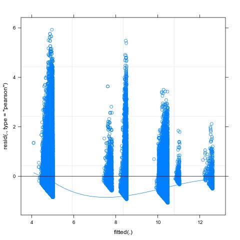
When I plot the residuals using: plot(mixed_eff_model, type = c('p', 'smooth'), the output is as follows:

I have two questions: 1. Does this indicate that the linear model is potentially misspecified? 2. How do I correct the model to account for this observation?

Answer 1

A couple of observations:

• From the output, it seems that you only have three groups for the grouping variable M. These are too few to meaningfully estimate the variance of the random effects you have included. Typically more than 10-20 groups are required to get stable estimates of the heterogeneity.
• The shape of the residuals suggests that you have heteroscedasticity with a smaller variance of the residuals for larger fitted values. Moreover, there are also some indications that perhaps your outcome Y has a lower bound.
• Some possible solutions are to account for the bounded nature of your outcome in case this is true, and investigate whether the heteroscedasticity is attributed to some of the predictors. The latter could be done using the lme() function from package nlme, which allows to specify a variance function via its weights argument.