Linear Regression: how to discern a possible correlation between observation errors from scatter plot

Question

The following is excerpted from An Introduction to Statistical Learning by Tibshiriani et. al. In page 66, they introduce the standard error for linear regression coefficients: $$Y = \beta_0+\beta_1X+\epsilon,\quad \epsilon \sim \mathcal N (0, \sigma)$$ $$SE(\hat \beta_0)^2 = \sigma^2 \Big[\frac{1}{n} +\frac{\bar x^2 }{\sum_{i=1}^n(x_i-\bar x)^2} \Big] $$ and $$SE(\hat \beta_0)^2 =\frac{\sigma^2}{\sum_{i=1}^n(x_i-\bar x)^2}.$$ The passage then proceeds as below:

"For these formulas to be strictly valid, we need to assume that the errors $\epsilon_i$ for each observation are uncorrelated with common variance $σ^2$. This is clearly not true in Figure 3.1, but the formula still turns out to be a good approximation." Here is the figure:

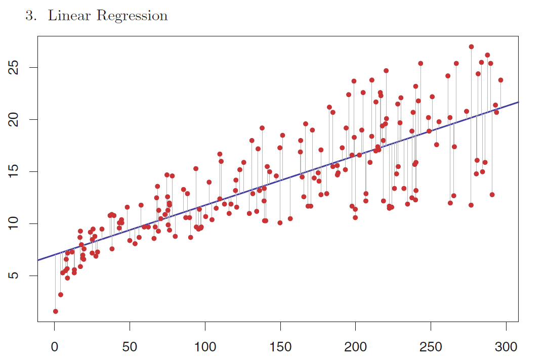
I understand that the assumption of independent errors can be quite unrealistic in many scenarios. But if some correlation is suspected, I would think of, for example, the Durbin-Watson test to detect it.

Now, first, what do the authors mean by "this" in the sentence "this is clearly not true"? Are they referring to the common variance assumption or to the uncorrelated errors assumption?

And in general, is it possible to detect correlation between observation errors from a scatter plot (particularly this one)?

Answer 1

Assuming that this is a plot of x vs. y, the common variance assumption is clearly off. There is much greater variance on the right side of the plot than the left, indicating that y is less well predicted by x as x increases (at least in absolute terms).

You could do various tests for heteroscedasticity, but I suggest using both OLS regression and a model that does not assume homoscedasticity (such as quantile regression) and seeing if median regression gives very similar results to mean regression - if the DV is symmetric. If the DV is asymmetric, you could choose a quantile that approximates the mean.