How could one estimate $Y = X\beta \times \epsilon$ with $\epsilon \sim \text{Beta}(a,b)$?

Question

Suppose the data generating process is $$Y_i=f(X_i)M_i.$$ where $M_i$~$Beta(a,b)$ and $f$ linear, for example,$f(X_i)=\alpha_0+\alpha_1X_i$. This is equivalent to $$M_i=Y_i/f(X_i).$$ I'm trying to think of someway to estimate $a,b$ and the $\alpha'$s. Do you have any suggestion?

I don't know if I have to go through Bayesian estimation.

Thanks in advance!

Answer 1

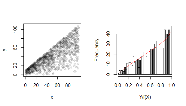
You might try to use find parameters by maximizing the likelihood function computationally (after finding some initial estimate for the parameters).

1. linear model estimate

2. compute parameters based on linear estimates and residuals

   In the code below I do this different and I assume $a=b$ and make use of $Y/f \sim Beta$. This has a problem that these values may not need to be limited in the range $(0,1)$. You could advance this step by making computations of the moments of the residuals and relate those to $a$ and $b$ (You should do this in order to make the convergence in the next step work better. I didn't do it because it involves annoying equations.)

3. perform computational optimization.

The code below shows a rough start for how this could work.

There are several issues:

• Values $Y_i/f(X_i)$ may reach outside the range $(0,1)$.
• The algorithm may not always converge well (With adaptations you can make it work well. The code before the edit used scaling of parameters. But more stable is the code after the edit, which uses segregated steps and solves the the problem as two nested optimizing functions).
• The error in the parameters is correlated. You can simultaneously increase the linear part $f(X)$ and decrease the mean of $M_i$, and this will give a roughly similar result. So while you can approximate the distribution well, the parameters may not be very meaningful and have a large error. (although when you test the model a few times the result does seem to turn out very close each time)

Quantile regression might be another angle to tackle this problem.

Furthermore, you can use various rough estimates instead of this computation. For instance a simple GLM model, not with a beta distribution but with some other distribution, might be sufficient for you to estimate the linear function $f$. How far these kind of approximations/simplifications can be made and whether they are sufficient for you, depends on the details of your problem.

example results:

True model
a = 2     b = 1      alpha_0 = 10     alpha_1 = 1  

Fit
a = 1.82  b = 0.93   alpha_0 = 10.02  alpha_1 = 1.00

example code:

library(betareg)
set.seed(1)

# create modelled data
n <- 10^3
x <- runif(n,0,100)
m <- rbeta(n,2,1)
X <- cbind(rep(1,n),x,x^2)
f <- X %*% c(10,1,-0.005)
y <- f*m
colnames(X) <- c("1","x","x^2")

# likelihood to optimize
loglik <- function(par,dat=dat) {
  # linear model pars
  #bt0 <- par[1]
  #bt1 <- par[2]
  
  # ratio Y/f(X) which should relate to beta distributed var
  f <- dat[,-1] %*% par
  yf <- dat[,1] / f
  
  #to prevent values outside (0,1) or values condensing in one point
  neg_penalty <- which(abs(yf-0.5) < 0.4999)
  
  # fit beta distribution to Y/f(x)
  # note under the hood betareg is a call to optim
  modfit <- betareg(yf[neg_penalty] ~ 1, link ="log")
  a <-    exp(modfit$coefficients$mean)  * modfit$coefficients$precision
  b <- (1-exp(modfit$coefficients$mean)) * modfit$coefficients$precision
  
  # return loglikelihood or penalty
  penalty_size <- length(dat[-neg_penalty,1])
  if (penalty_size == 0) {
    result <- -modfit$loglik + sum(log(f)) 
        # the sum(log(f)) term is because we actually do not wish the
        # probability for yf but instead the probability for y which relates
        # to a scaled beta distribution and this scaling factor occurs in the density as log(f)
  } else {
    result <- penalty_size*10^6
  }
  result
}

# data
dat <- cbind(y,X)

# start condition
mod <- lm(y ~ 0+X)
par <- c(2*mod$coefficients)  # we assume that the starting line is twice the mean

# optimize
p <- optim(par, loglik, dat=dat, control = list(trace=2, maxit=10^3)) 
p

# outcome
p$par
loglik(par,dat)
loglik(p$par,dat)

yf <- dat[,1] / (X %*% p$par)
modfit <- betareg(yf ~ 1, link ="log")
parfin <- c(exp(modfit$coefficients$mean)*modfit$coefficients$precision,
         (1-exp(modfit$coefficients$mean))*modfit$coefficients$precision,
         p$par)

# view result
plot(x, y, 
     pch=21, col=rgb(0,0,0,0.1),bg=rgb(0,0,0,0.1))


sig <- 0.02
brks <- seq(0,1,sig)
hist(yf, breaks = brks,sig,xlim=c(min(hf),max(hf)),xlab = "Y/f(X)",main="")
lines(brks,dbeta(brks, parfin[1],parfin[2])*n*sig,col=2)

parfin