Confusion about Anderson-Darling test

Question

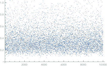
The Anderson-Darling test statistic is $$ A^2 := n \int_{-\infty}^{\infty} \frac{(F_n(x)-F(x))^2}{F(x)(1-F(x))} \, \mathrm{d}F(x) $$ We know that the samples $$ Z(x) := \frac{\sqrt{n}(F_{n}(x) - F(x))}{F(x)(1-F(x))} \to \mathcal{N}(0,1) $$ and hence if we convert the expression for $A^2$ into a quadrature sum we obtain $$ A^2 \approx \sum Z(x_i)^2 F'(x_i) w_i $$ Presumably $F'(x)$ decays in some way (say, as a bell curve), so that the the following argument is not totally rigorous, but in any case, we make the approximation that $$ A^2 \approx C\sum Z(x_i)^2 $$ we see that the statistic is the sum of squares of $\mathcal{N}(0,1)$ samples and hence is itself highly variable. Assuming roughly $k$ samples of the quadrature sum are located near the maximum of the pdf, then $A^2 \sim \chi(k)$, and $A^2$ has variance $k$, but damped a bit by the shape of the pdf. Even if this argument is not rigorous, we can see that the test is itself is highly variable in this simulation, created with the following Mathematica command:

ListPlot[Table[
  AndersonDarlingTest[RandomVariate[NormalDistribution[], n], 
   Automatic, "TestStatistic"], {n, 2, 10000, 1}]]

Moreover, it doesn't improve with n. You have the expectation that if $F_{n} \to G \ne F$, then $A^2$ should approach some finite positive limit, and if $F_n \to F$, then $A^2 \to 0$, and hence you're convinced that the distance measure induced by the integral shows that they are the same. But that's not the case! If $F_n\to G$, then the integral diverges, and $F_n \to F$, the integral bounces around. And maybe you say what's the problem? I can distinguish between a bounded random sequence and an unbounded one. But that's only if you have the ability to arbitrarily draw more and more data. That's not the case in many circumstances.

However, $A^2/n \to 0$ iff $F_n \to F$, and $A^2/n \to \epsilon > 0$ whenever $F_n \to G \ne F$. So why don't we consider the quantity $A^2/n$ instead of $A^2$ in the Anderson-Darling test?

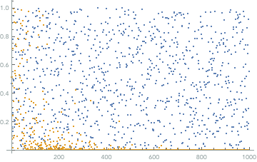
Edit: The conversion to the $p$-value seems especially dubious here. You'll get a different p-value every time if the hypothesis is true, and that $p$-value looks uniformly distributed on $[0,1]$ independent of $n$. Fortunately if it's false and $n \to \infty$ the $p$-value does seem to drop to zero.

Here's the code:

ListPlot[{Table[
   AndersonDarlingTest[RandomVariate[NormalDistribution[0.0, 1], n], 
    NormalDistribution[0, 1], "PValue"], {n, 2, 1000, 1}], 
  Table[AndersonDarlingTest[
    RandomVariate[NormalDistribution[0.2, 1], n], 
    NormalDistribution[0, 1], "PValue"], {n, 2, 1000, 1}]}]

Answer 1

To start, I think you are missing the point of hypothesis testing. We wish to have a test statistic, T, that is some function of the data. Under the assumption the null hypothesis is true, this T should be some underlying null distribution which, under the alternative, it will not be. There, we can compute notions of "probability under the assumption the null hypothesis is true if our statistic is more extreme in the direction of the alternative." Having it converge to point instead of a distribution will not allow us to do this.

Also, your expansion is not quite right because the Z's are in fact very correlated, so sum would not be chi square with n degrees of freedom.

Further, your p value should be uniformly distributed under the null hypothesis. If you observe X under the null distribution, then compute its cdf, it will in fact be uniformly distributed.