Number of events in a segment if waiting times are drawn from a mixture of two exponential distributions

Question

What is the probability for $n$ events to occur over a period of time $t$, if the duration of each event is a random variable distributed as a mixture of two exponential distributions, one with the average duration $\tau_1$ and the probability $p$ and the other with average duration $\tau_2$ and the probability of $(1-p)$?

For example, we have a doctor who has both healthy patients and sick patients waiting in line, with the relative fractions of 80% and 20%. Healthy patients take on average 5 minutes per visit, sick ones take one hour, with the actual durations distributed exponentially. How many times would the doctor's door open during a period of half an hour?

Answer 1

Part 1: fixed waiting times

What is the probability for $n$ events to occur over a period of time $t$, if the duration of each individual event is $\tau_1$ with the probability $p$ and $\tau_2$ with the probability of $(1-p)$?

There is a correspondence between waiting time and number of events per time

see: https://stats.stackexchange.com/a/450135/164061

For time $t$ and number $n$ you get: $$\begin{array}{ccc} \overbrace{P(N \geq n| t)}^{\text{this is what you are looking for}} &=& \overbrace{P(T \leq t|n)}^{\text{we will express this instead}} \\ {\small\text{prob. counts $n$ or above given time $t$}} &=& {\small\text{prob. waiting time below $t$ given counts $n$}} \end{array} $$

In words: the probability to get more than $n$ counts within time $t$ equals the probability to need less than $t$ time to get $n$ counts. For all cases that got $n$ or more cases within time $t$, they must have had $n$ cases below time $t$ and none of them had $n$ cases in time $t$ or above.

and this relates many distributions.

Distribution of                 Distribution of 
Waiting time between events     number of events

Exponential                     Poisson
Erlang/Gamma                    over/under-dispersed Poisson  
Geometric                       Binomial
Negative Binomial               over/under-dispersed Binomial

---

So let's express the alternative: What is the probability for $n$ events to take time $t$ or less?

• The distribution of time for $n$ events can be expressed as a scaled and shifted binomial distribution. For $n$ events we have the number of events of type '1' and the events of type '2' which is binomial distributed.

  $$P(N_1 = n_1) = {{n}\choose{n_1}} p^{n_1} (1-p)^{n-n_1}$$

  and CDF

  $$P(N_1 \leq n_1) = I_q(n-n_1,1+n_1)$$

  where $I$ is the regularized beta function.

• Now we need to convert this to time which is quick step. The time $t$ is equal to $$t=\tau_1 n_1 + \tau_2 (n-n_1)$$ or $$t=(\tau_1-\tau_2) n_1 + \tau_2 n$$

  So the time to handle $n$ patients is basically a scaled and shifted binomial variable.

• So, to know the probability for $N$ events being less or equal to $n$ given time $t$, we compute the probability for the probability that time $T$ given $n$ is larger than $t$, and this we do with a binomial distribution (where we need to take into account a shift and scaling).

Step 2: exponentially distributed waiting times

with the actual durations distributed exponentially. How many times would the doctor's door open during a period of half an hour?

This will require some more steps...

...but it will follow the same lines. Convolute the individual waiting time distributions (in this case now it is a mixture of exponential distributions) to get the total waiting distributions, and then invert switch independent and dependent variables.

The main problem is now that a sum of different exponentially distributed variables (with different $\tau$) is not easily expressed/computed. So you are likely gonna use an approximate method, of which there are many variations (4 of them below of which 2 computed in the code).

The R-code below gives two examples

1. We can compute the distribution (and the related mean) by simulating the process a lot of time. In the code below this is done by adding exponential variables until the time exceeds 30 minutes. Then after doing this a lot of times we can draw a histogram of the distribution of the times that we can add exponential variables untill we exceed 30 minutes.

2. We can model the distribution as a continuous Markov process. And the distribution of the time $t$ until having $n$ patients is phase-type distributed. The transition matrix (for states 0,...,2k) has the form like (where $\lambda = 1/\tau$):

   $$\begin{bmatrix}{} 0& 0 & 0 & 0 & 0 & 0 & 0 \\ 0& -\lambda_1 & 0 & p_1 \lambda_1 & p_2 \lambda_1 & 0 & 0 \\ 0&0 & -\lambda_2 & p_1 \lambda_2 & p_2 \lambda_2 & 0 & 0 \\ 0&0&0& -\lambda_1 & 0 & p_1 \lambda_1 & p_2 \lambda_1 \\ 0&0&0&0& -\lambda_2 & p_1 \lambda_2 & p_2 \lambda_2 \\ \lambda_1&0&0&0&0& -\lambda_1 & 0 \\ \lambda_2&0&0&0&0&0& -\lambda_2 \end{bmatrix}$$

   which has repeated blocks like

   $$\begin{bmatrix}{} -\lambda_1 & 0 & p_1 \lambda_1 & p_2 \lambda_1 \\ 0 & -\lambda_2 & p_1 \lambda_2 & p_2 \lambda_2 \\ \end{bmatrix}$$

   The begin state is with fraction $p_1$ in $1$ and $p_2$ in $2$. The transitions will be going in steps from pairs to pairs, ie. from states $2k$ or $2k+1$ to states $2(k+1)$ or $2(k+1)+1$, and the rates by which a step is made will depend on whether the current state is odd or even.

   In the last two lines

   $$\begin{bmatrix}{} \lambda_1&0&0&0&0& -\lambda_1 & 0 \\ \lambda_2&0&0&0&0&0& -\lambda_2 \end{bmatrix}$$

   The transition goes to the absorbing state 0.

Not worked out in this answer and the code below is an exact expression of the distribution function

3. Possibly there might be a way to express the waiting time for $n$ patients as a mixture of gamma distributions by expressing the characteristic function of the distribution of the waiting time for $n$ patients

   $$\varphi_{T \vert n}(t) = \left[ \frac{p_1}{1 - i \tau_1 t} + \frac{p_2}{1 - i \tau_2 t} \right]^n$$

   in terms of a mixture of gamma distributions.

Also we may use a normal distribution approximation and a Taylor series approximation. See here.

4. If the waiting time for a single event has finite variance then the conditions of the CLT are fulfilled and the waiting time for more events will be asymptotically normal distributed. Then we can model the distribution of $m$ as an approximately normal distribution :

   $$P(M \leq m \vert x) \approx \Phi \left( \frac{m-x\theta_1}{\sqrt{x}\theta_2} \right)$$

   Note that the CLT is more precisely $\sqrt{x}(M/x-\theta_1) \sim N(0,\theta_2)$ so this is where the distribution of $M$ and not $\sqrt{x}(M/x-\theta_1)$ may still differ from a normal distribution. But the scaled variable $M/x$ is approaching a normal dsitribution.

   and we can convert this into

   $$P(X < x \vert m) = P(M > m \vert x) \approx \Phi \left( \frac{x-m/\theta_1}{\sqrt{x}\theta_2/\theta_1} \right) \underbrace{\approx \Phi \left( \frac{x-m/\theta_1}{\theta_2\sqrt{m/\theta_1^3}} \right)}_{\text{Taylor series approximation}} $$

   where $\theta_1$ and $\theta_2$ are respectively the mean and standard deviation of the waiting time for a single event.

   In our case the mean waiting time is

   $$\theta_1 = p_1 \tau_1 + p_2 \tau_2$$

   and the standard deviation of the waiting time of a single event is (see here to derive the formula)

   $$\theta_2 = \sqrt{2 p_1 \tau_1^2 + 2 p_2 \tau_2^2 - (p_1 \tau_1 + p_2 \tau_2)^2 }$$

   This approximation is not working well for small values of patients though, because in that case the approximation with a normal distribution is not a good approximation.

---

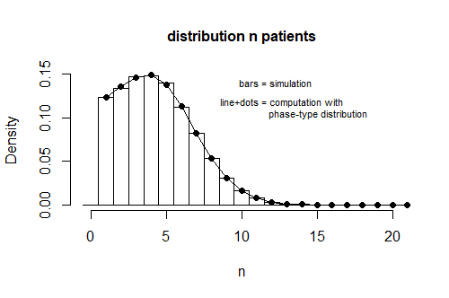
Example image for case 1 and 2:

Simulation and computation of the distribution of patients in half an hour. The mean/average will be around 4.38/3.38, depending on whether you count the times the door opens for a patient entering/leaving.

Example code:

######################

library(actuar)
set.seed(1)

## parameters for simulation
n <- 10^5
nt <- rep(0,n)

## parameters describing problem 
tl <- 30
t1 <- 5
t2 <- 60
l1 <- 1/t1
l2 <- 1/t2
p1 <- 0.8
p2 <- 0.2

##
## simulate patients
##
for (i in 1:n) {
  t = 0
  while (t <= tl) {
    lambda = l2 + (l1-l2) * rbinom(1,1,p1) 
    t = t + rexp(1,lambda)
    nt[i]=nt[i]+1
  }

}

##
## computing patients with phase-type distribution
##

#star transition matrix
T <- rbind(c(-l1,  0   ),
           c( 0   , -l2))
pi <- c(p1,p2)
# computing time within 30 min
cump <- pphtype(30,pi,T)


for (i in 1:20)
{
  # extending transition matrix by 2 rows
  T <- rbind(c(-l1,  0  , p1*l1 , p2*l1, rep(0,length(T[,1])-2)),
             c( 0 , -l2 , p1*l2 , p2*l2, rep(0,length(T[,1])-2)),
             cbind(0,0, T)
            )
  pi <- c(pi,0,0)
  # computing time within 30 min
  cump <- c(cump,pphtype(30,pi,T))
}

ps <- (-diff(c(1,cump)))

##
## plotting histogram
##
h <- hist(nt, breaks = seq(-0.5,20.5,1),
          main = "distribution n patients", freq  = FALSE, xlab = "n")

### computed probabilities for bn patients
lines(ps)
points(ps, col = 1, bg = 1, pch = 21)


## expressing mean
sum(h$density*h$mids)
sum(ps*c(1:21))
tl/(p1*t1+p2*t2)+1

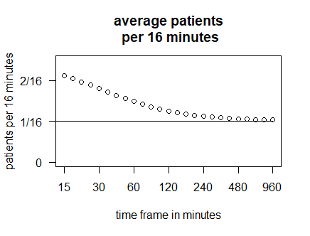
Example image for case 2:

With this code we can compute/approximate the discrepancy between the expected number of patients and the inverse of the expected waiting time (1/16). The longer the time frame the closer the two will be.

### placing the computation with phase-type distribution in a function
ptime <- function(minutes, ncomp = 100, 
                  t1 = 5, t2 = 60, p1 = 0.8, p2 = 0.2) {

  l1 <- 1/t1
  l2 <- 1/t2

  #star transition matrix
  T <- rbind(c(-l1,  0   ),
             c( 0   , -l2))
  pi <- c(p1,p2)
  # computing time within minutes min
  cump <- pphtype(minutes,pi,T)


  for (i in 1:ncomp)
  {
    # extending transition matrix by 2 rows
    T <- rbind(c(-l1,  0  , p1*l1 , p2*l1, rep(0,length(T[,1])-2)),
               c( 0 , -l2 , p1*l2 , p2*l2, rep(0,length(T[,1])-2)),
               cbind(0,0, T)
    )
    pi <- c(pi,0,0)
    # computing time within 30 min
    cump <- c(cump,pphtype(minutes,pi,T))
  }

  ps <- (-diff(c(1,cump)))
  ps
}


### computing distributions for different times
meanout <- c()
cmins <- 15*2^seq(0,6,0.25)
nsim <- 150
plot(-100,-100, xlim = c(0,nsim), ylim = c(0,0.3))
for (mins in cmins) {
  ps <- ptime(mins, ncomp = nsim)
  lines(0:nsim,ps)
  meanout <- c(meanout,sum(ps*c(0:nsim))/mins)
}

### plotting the means
plot(cmins,meanout, ylim = c(0,0.15), 
     main = "average patients\n per minute",
     xlab = "time frame in minutes", 
     ylab = "patients per minute")
lines(c(0,max(cmins)),rep(1/(p1*t1+p2*t2),2))

Answer 2

The distribution of waiting times you describe is a hyperexponential distribution. See the Wikipedia entry for details.

each $Y_i$ is an exponentially distributed random variable with rate parameter $\lambda_i$, and $p_i$ is the probability that $X$ will take on the form of the exponential distribution with rate $\lambda_i$

The expected value of wait time is simply:

$$E[X]=\sum_{i=1}^n \tfrac{p_i}{\lambda_i}$$

In your example, the average waiting time is $\tfrac{0.8}{1/5}+\tfrac{0.2}{1/60}=16$ minutes. The expected number of patients in a half-hour is $30/16=1.875$

Edit: I believe the final calculation for the expected number of patients per half-hour is correct for a random half-hour period but not necessarily the first half-hour. That is, if we look at a random half-hour period throughout the day it will work, but if we look at the first half-hour when the first patient arrives, or if we're assuming a patient arrives right at the beginning of the half-hour, then the answer will be different. This is because the hyperexponential distribution does not exhibit the memoryless property.