Best practices in the selection of distance metric and clustering methods for gene expression data

Question

I have been reading about this on various channels including here and Stack Exchange, but I'm still not sure how to choose the best approach for clustering gene expression data. As a Ph.D. molecular biologist (with no in-depth Math/Statistics background), I'm looking for a set of guidelines that one should follow for clustering. I will set the stage below for my problem and provide a reproducible example, but as a background study, I did the following which wasn't really helpful:

• I performed extensive searches in SE/SO and talked to various bioinformaticians on this issue. I understand the general differences between various hclust methods and distance metrics. While I realize this my question sounds like a common one, I couldn't exactly find satisfying answers to understand the best approach for clustering RNAseq and microarray data. It seems like a lot of people have their favorite "way" of doing things and not much thought goes into understanding which distance metric/clustering method should be used and why.

• I read several posts about the choice of clustering methods including, this, this, this, this, and many others

My goal is to cluster samples based on their gene expression profiles and find real patterns within the dataset. Secondarily, I would also like to perform hierarchical clustering analysis for genes (variables in columns).

Couple words on data structure: Like many common RNAseq data, my real RNAseq dataset is composed of hundreds of observations (samples in rows) and thousands of genes (variables in columns). Distribution of gene expression values across samples may or may not be normal-like and the expression ranges can differ greatly. By using established methods (such as limma or DEseq2), I generated normalized counts in log2 scale (normalization based on the total number of transcript counts). I would like to perform clustering by using both the entire dataset and a subset of genes that I'm interested in.

I have a lengthy reproducible example below, please take a look to follow my questions (especially the comparisons towards the end are relevant).

My specific question is:

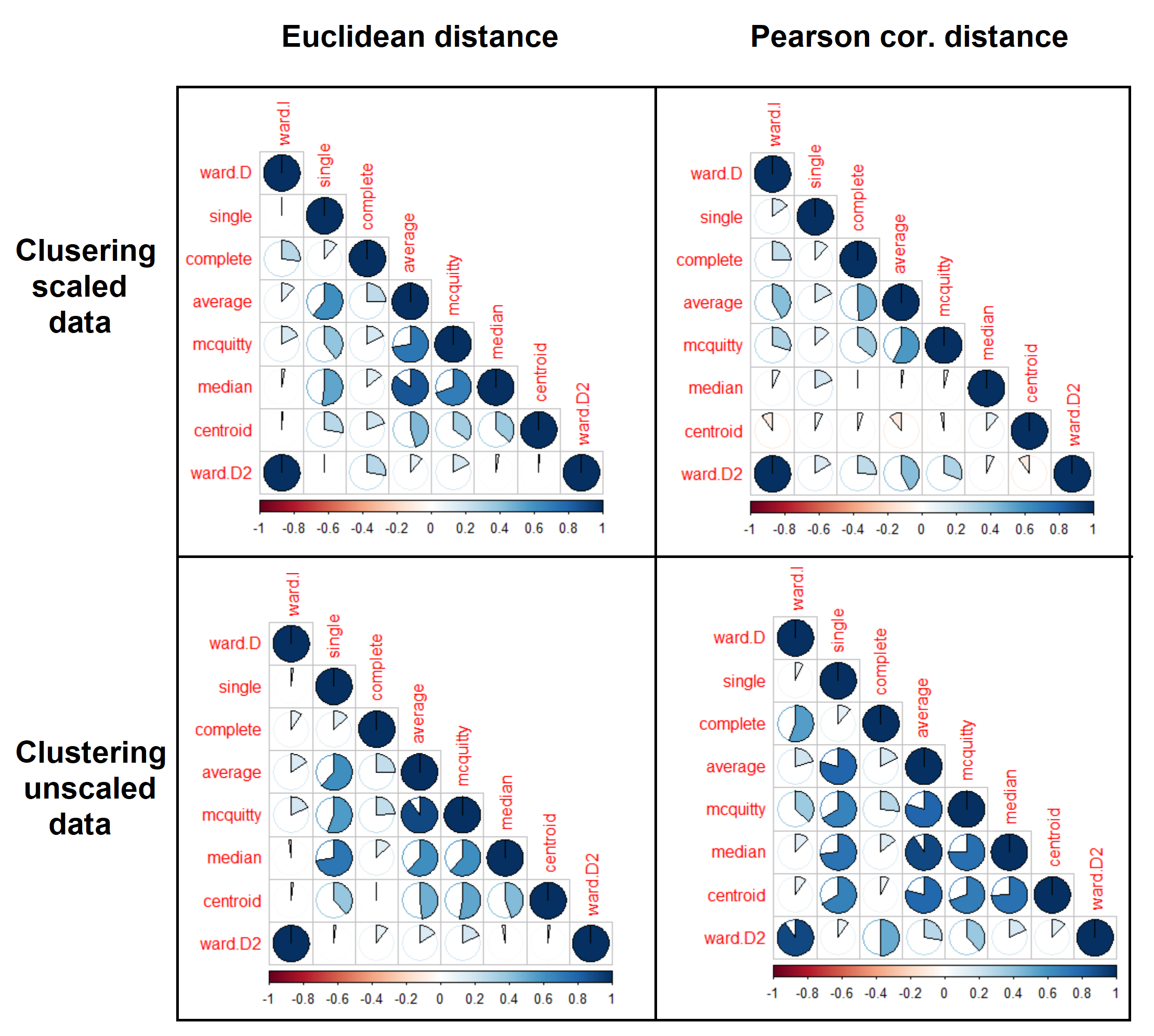
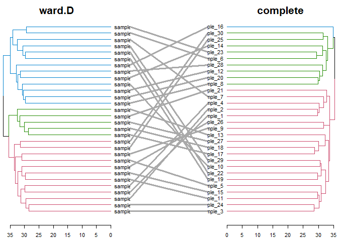
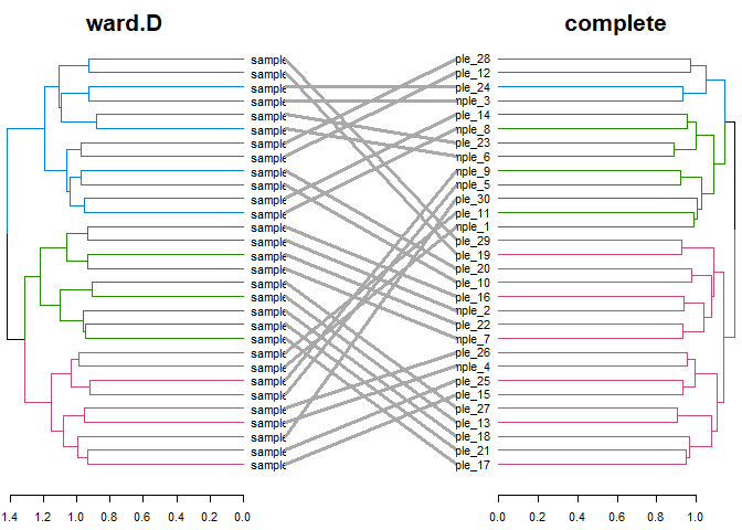
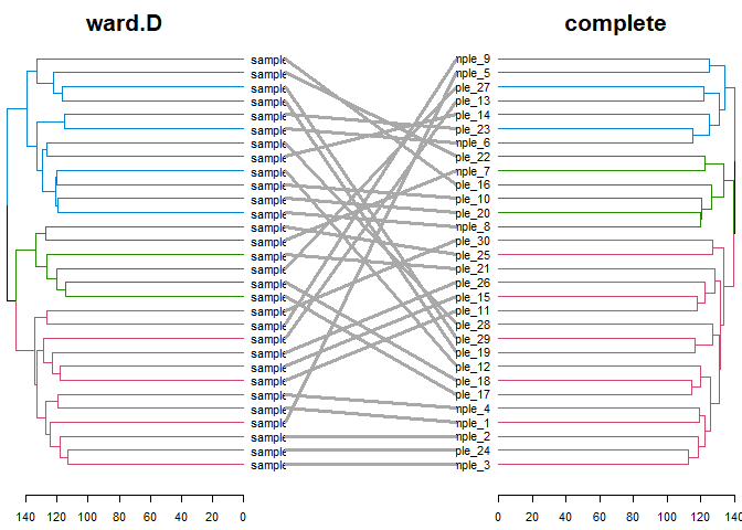
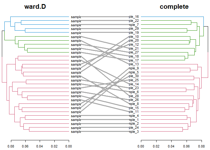
What are the most appropriate distance metric and hierarchical clustering methods for clustering samples (observations) and why? I performed hclust with different methods below on mock data (mtx) and the results were highly variable. Please see the cluster tree comparisons and overall correlation among clustering methods. I'm not sure which one to believe in.

Sorry for the long post, but in summary, I'm trying to understand the most appropriate approach for clustering gene expression data (applicable to both RNAseq and microarray) to see real patterns while avoiding patterns that might occur due to random chance.

Reproducible example

Simulate data

library(reprex)
library(pheatmap)
library(dendextend)
library(factoextra)
library(corrplot)
library(dplyr)



set.seed(123)

mtx_dims <- c(30, 500)

mtx <- matrix(rnorm(n = mtx_dims[1]*mtx_dims[2], mean = 0, sd = 4), nrow = mtx_dims[1])

mtx[, 1:10] <- mtx[ , 1:10] + 10  # blow some genes off-scale
mtx[, 11:20] <- mtx[, 11:20] + 20 
mtx[, 21:30] <- mtx[, 11:20] + 30 
mtx[, 31:40] <- mtx[, 11:20] + 40 
mtx[, 41:50] <- mtx[, 11:20] + 50 


rownames(mtx) <- paste0("sample_", 1:mtx_dims[1])
colnames(mtx) <- paste0("gene_", 1:mtx_dims[2])

rowannot <- data.frame(sample_group = sample(LETTERS[1:3], size = mtx_dims[1], replace = T))
rownames(rowannot) <- rownames(mtx)


unscaled_mtx <- mtx

mtx <- scale(mtx)

Exploratory heatmap/clustering

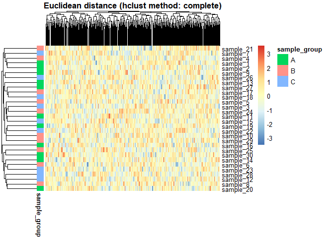
pheatmap(mtx,
         scale = "none",
         clustering_distance_rows = "euclidean",
         clustering_distance_cols = "euclidean",
         clustering_method = "complete",
         main = "Euclidean distance (hclust method: complete)",
         annotation_row = rowannot,
         show_colnames = F)

pheatmap(mtx,
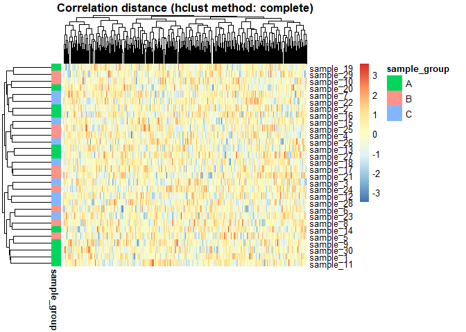
         scale = "none",
         clustering_distance_rows = "correlation",
         clustering_distance_cols = "correlation",
         clustering_method = "complete",
         main = "Correlation distance (hclust method: complete)",
         annotation_row = rowannot,
         show_colnames = F)

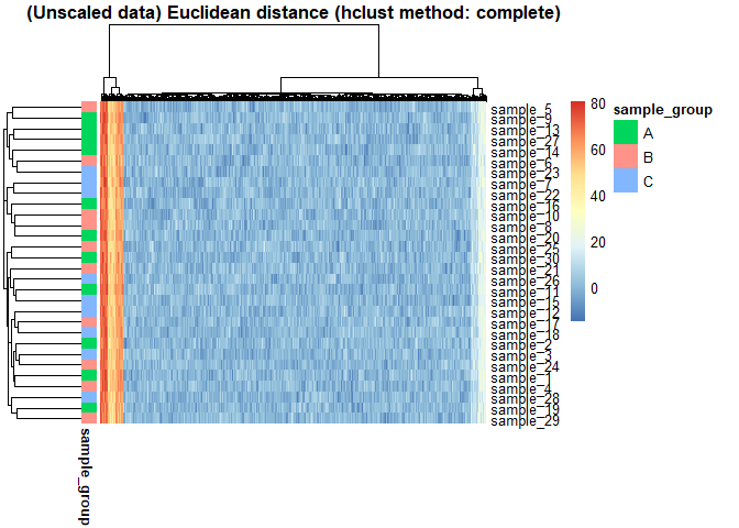
pheatmap(unscaled_mtx,
         scale = "none",
         clustering_distance_rows = "euclidean",
         clustering_distance_cols = "euclidean",
         clustering_method = "complete",
         main = "(Unscaled data) Euclidean distance (hclust method: complete)",
         annotation_row = rowannot,
         show_colnames = F)

Scaled mtx clustering

Euclidean Distance

d_euc_mtx <- dist(mtx, method = "euclidean")    


hclust_methods <- c("ward.D", "single", "complete", "average", "mcquitty", 
                    "median", "centroid", "ward.D2")

mtx_dendlist_euc <- dendlist()

for(i in seq_along(hclust_methods)) {


    hc_mtx <- hclust(d_euc_mtx, method = hclust_methods[i])   

    mtx_dendlist_euc <- dendlist(mtx_dendlist_euc, as.dendrogram(hc_mtx))
}

names(mtx_dendlist_euc) <- hclust_methods


mtx_dendlist_euc_cor <- cor.dendlist(mtx_dendlist_euc, method_coef = "spearman")


corrplot(mtx_dendlist_euc_cor, "pie", "lower")

mtx_dendlist_euc %>% dendlist(which = c(1,3)) %>% ladderize %>% 
    set("branches_k_color", k=3) %>% 
    tanglegram(faster = TRUE)

Pearson correlation distance

d_cor_mtx <- get_dist(mtx, method= "pearson", diag=T, upper=T)



mtx_dendlist_cor <- dendlist()

for(i in seq_along(hclust_methods)) {

    hc_mtx <- hclust(d_cor_mtx, method = hclust_methods[i])   

    mtx_dendlist_cor <- dendlist(mtx_dendlist_cor, as.dendrogram(hc_mtx))
}

names(mtx_dendlist_cor) <- hclust_methods

mtx_dendlist_cor_cor <- cor.dendlist(mtx_dendlist_cor, method_coef = "spearman")


corrplot(mtx_dendlist_cor_cor, "pie", "lower")

mtx_dendlist_cor %>% dendlist(which = c(1,3)) %>% ladderize %>% 
    set("branches_k_color", k=3) %>% 
    tanglegram(faster = TRUE)

Unscaled mtx clustering

Euclidean Distance

d_euc_mtx <- dist(unscaled_mtx, method = "euclidean")    


hclust_methods <- c("ward.D", "single", "complete", "average", "mcquitty", 
                    "median", "centroid", "ward.D2")

mtx_dendlist_euc <- dendlist()

for(i in seq_along(hclust_methods)) {


    hc_mtx <- hclust(d_euc_mtx, method = hclust_methods[i])   

    mtx_dendlist_euc <- dendlist(mtx_dendlist_euc, as.dendrogram(hc_mtx))
}

names(mtx_dendlist_euc) <- hclust_methods




mtx_dendlist_euc_cor <- cor.dendlist(mtx_dendlist_euc, method_coef = "spearman")


corrplot(mtx_dendlist_euc_cor, "pie", "lower")

mtx_dendlist_euc %>% dendlist(which = c(1,3)) %>% ladderize %>% 
    set("branches_k_color", k=3) %>% 
    tanglegram(faster = TRUE)

Pearson correlation distance

d_cor_mtx <- get_dist(unscaled_mtx, method= "pearson", diag=T, upper=T)


mtx_dendlist_cor <- dendlist()

for(i in seq_along(hclust_methods)) {

    hc_mtx <- hclust(d_cor_mtx, method = hclust_methods[i])   

    mtx_dendlist_cor <- dendlist(mtx_dendlist_cor, as.dendrogram(hc_mtx))
}

names(mtx_dendlist_cor) <- hclust_methods


mtx_dendlist_cor_cor <- cor.dendlist(mtx_dendlist_cor, method_coef = "spearman")


corrplot(mtx_dendlist_cor_cor, "pie", "lower")

mtx_dendlist_cor %>% dendlist(which = c(1,3)) %>% ladderize %>% 
    set("branches_k_color", k=3) %>% 
    tanglegram(faster = TRUE)

Cluster validation (using scaled matrix)

# The goal of this is to understand how many clusters are predicted by different
# clustering methods and index scores.

suppressPackageStartupMessages(library(NbClust))


indices <- c("kl", "ch", 
             # "hubert", "dindex",  # take longer to compute and create graphical outputs
             "ccc", "scott", "marriot", "trcovw", 
             "tracew", "friedman", "rubin", "cindex", 
             "db", "silhouette", "duda", "pseudot2", 
             "beale", "ratkowsky", "ball", "ptbiserial", 
             "gap", "frey", "mcclain", "gamma", "gplus", 
             "tau", "dunn","hartigan", "sdindex",  "sdbw")

cl_methods_nb <- c("ward.D", "ward.D2", "single", "complete", "average", "mcquitty", "median", "centroid", "kmeans")

val_res <- list()

for(j in cl_methods_nb){

    for(i in indices) {

        # message(i)

        tryCatch({
            val_res[[paste(j,i, sep = "_")]] <- NbClust(data = mtx, diss = d_cor_mtx, 
                                                        distance = NULL, method = j,
                                                        index=i, max.nc = 6)}, 
            error=function(e){
                # message(paste(j, i, "failed"))
            })

    }

}
#> Warning in pf(beale, pp, df2): NaNs produced

#> Warning in pf(beale, pp, df2): NaNs produced
#> [1] "Frey index : No clustering structure in this data set"
#> [1] "Frey index : No clustering structure in this data set"



val_res_nc <- data.frame()

for(i in names(val_res)){

    method_name <- gsub("_.*", "", i)
    index_name <- gsub(".*_", "", i)

    if(!"Best.nc" %in% names(val_res[[i]])) next

    df_int <- data.frame(method_name = method_name,
                         index_name = index_name,
                         best_nc = val_res[[i]][["Best.nc"]][1])

    val_res_nc <- rbind(val_res_nc, df_int)

}


# Breakdown of cluster number as predicted various clustering
# methods and validation indices
summary(as.factor(val_res_nc$best_nc))
#>  1  2  3  4  5  6 
#>  3 71 20  9 21 63

# Tabulate data
head(
    val_res_nc %>%
         group_by(method_name, index_name) %>%
         summarize(best_nc), 10
    )
#> # A tibble: 10 x 3
#> # Groups:   method_name [1]
#>    method_name index_name best_nc
#>    <fct>       <fct>        <dbl>
#>  1 ward.D      kl               4
#>  2 ward.D      ch               2
#>  3 ward.D      cindex           6
#>  4 ward.D      db               6
#>  5 ward.D      silhouette       6
#>  6 ward.D      duda             5
#>  7 ward.D      pseudot2         5
#>  8 ward.D      beale            5
#>  9 ward.D      ratkowsky        6
#> 10 ward.D      ball             3

Correlation among hclust methods

Answer 1

This will probably not be the answer you want or expect, but this is how I see these things.

Clustering problem

Clustering, to a degree, is almost always a subjective procedure. You decide how you want to group different elements together, then choose a distance metric that satisfies your wishes, and then follow the procedures.

Here is a short example - imagine we want to cluster these animals into groups:

We can try different distances (based on how many legs they have, if they can swim or not, how high they are, their color) and all of the metrics would give different clusters. Can we say that some of them are correct and others incorrect? No. Does question "which result should I believe" makes sense? Also no.

RNA expression data

Same thing is happening with your example.

Imagine you want to group distinct genes into clusters. Immediately questions arise:

1) Questions about the distance measure: should genes that show the same pattern, but have different levels of overall expression go into the same group (correlation based distance) or different groups (difference based distance)? Is the pattern more important the the overall expression level ? If two genes anti-correlate does that mean they are related and be in the same group, or in different groups (does sign matter)? Should larger deviations be "punished" more (euclidean distance), or all magnitudes of difference are equally important (manhattan distance)?

2) Questions about the linkage function: do I want all the elements within one group to be at most "X" distance apart (complete linkage)? Or do I want to group genes under the same cluster if there is a chain of small changes that lead from one profile to another (single linkage)? etc.

These are the questions that practitioner has to answer in order to get a sensible result that he can later interpret. All of the above options can have biological meaning behind them. In one case you would get a cluster of genes that show similar levels of expression, in another case - a cluster of genes that show similar trends. There is no one way of doing it an no reason to think that you should believe one result and doubt the others. It may sound cliche but in a sense one has to know what he or she wants to do before he start doing it.

I think the correct way to be looking at this is that one should prefer one method in one situation and another method in a different situation.

Some possibilities

Now let's imagine we care about the following things:

1. we want to group genes if they are linearly related (increase or decrease among the same individuals).
2. we do not care about the magnitude differences between two genes (since they can be expressed at different levels, but still be related).

One possibility to satisfy the above is to use absolute correlation level as distance: $1 - |cor(gene_{1}, gene_{2})|$.

Then after we create the dendrogram we want:

1. to create groups so that all the elements within the group are correlated with one another by at least |0.7|.

For this we would pick "complete" linkage and cut the tree at the height of 0.3 (remember the distance is one minus correlation value).

Questions and advice

Now with the above context, here are the answers to the questions:

What are the most appropriate distance metric and hierarchical clustering methods for clustering samples (observations) and why?

The most appropriate distance will depend on the situation. If you want to group samples/genes by their overall expressions - you have to use one distance. If you want to group them by patterns - another distance.

I performed hclust with different methods below on mock data (mtx) and the results were highly variable. I'm not sure which one to believe in.

All of them are mostly equally believable. Since they all tried to achieve slightly different things, the results obtained were also different.

I'm trying to understand the most appropriate approach for clustering gene expression data (applicable to both RNAseq and microarray) to see real patterns while avoiding patterns that might occur due to random chance.

Avoiding patterns that arise because of chance, or worse, because of technical reasons (i.e. samples were done in batches) is not easy.

For noise I would advice to not scale your features (genes). Scaling would bring real signal and noise to the same level, which might have an influence on the result.

For the technical part - I would make sure that the groups obtained by clustering procedure do not follow the pattern of some technical parameter (i.e. samples done on batch1 are in one cluster and samples done on batch2 - in another cluster). If you find that this is the case, such batch effects will potentially have a huge influence on both: sample clusters and gene clusters.

Another thing you might try (when clustering genes for example) is to look for biological meaning behind the clusters. If you find that genes within one cluster have some common ontology terms that might provide additional confidence that the clusters you found are meaningful and not just noise.

Finally, it seemed like you want to try using only the genes that showed differences between some groups for your clustering. This is quite a pointless exercise (in my opinion), because it is quite clear what the result will look like: your two groups that you were comparing are bound to be separated, even if the procedure was performed on randomly generated numbers.