Random Forest - Variable Importance Plot Interpretation

Question

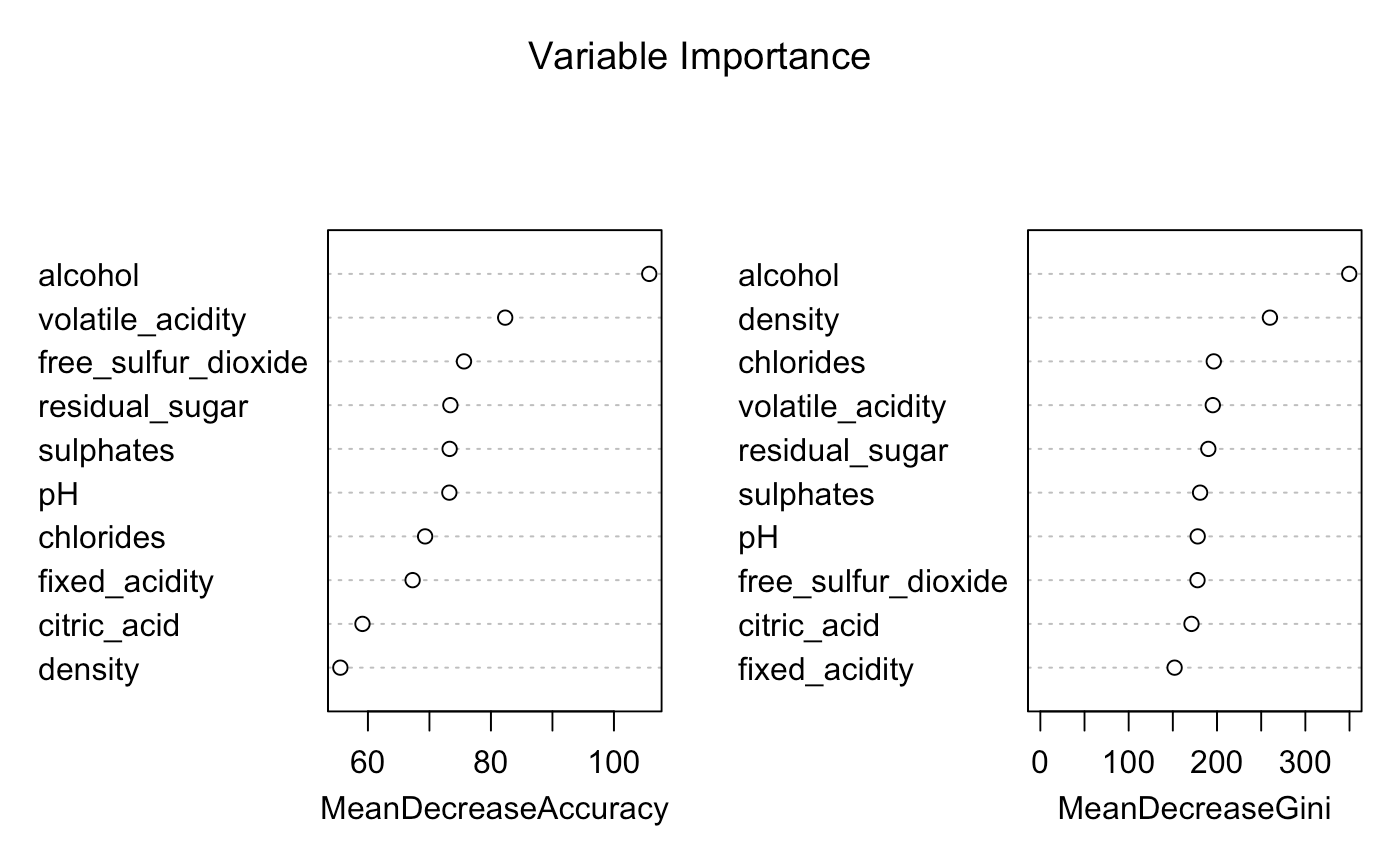
After modeling my Random Forest on my full dataset and the necessary predictor variables I am producing the below variable importance plot.

I'm currently trying to wrap my head around how to interpret these plots? It is obvious to me that alcohol is the more important predictor when it comes to model results, and without it, the model accuracy will decrease. However, how can I interpret these values based on their Mean Decrease Accuracy and Mean Decrease Gini?

Data set can be found here.

Current Code:

wine=read.csv("wine_dataset.csv")
wine$quality01[wine$quality >= 7] <- 1
wine$quality01[wine$quality < 7] <- 0
wine$quality01=as.factor(wine$quality01)
summary(wine)
num_data <- wine[,sapply(wine,is.numeric)]
hist.data.frame(num_data)

set.seed(8, sample.kind = "Rounding") #Set Seed to make sure results are repeatable
wine.bag=randomForest(quality01 ~ alcohol + volatile_acidity + sulphates + residual_sugar + 
    chlorides + free_sulfur_dioxide + fixed_acidity + pH + density + 
    citric_acid,data=wine,mtry=3,importance=T)    #Use Random Forest with a mtry value of 3 to fit the model

wine.bag #Review the Random Forest Results
plot(wine.bag) #Plot the Random Forest Results
varImpPlot(wine.bag)

I'm noticing some Mean Decrease Accuracy values over 100 and that is throwing me off.

Any tips would be appreciated.

Answer 1

Ok so the first plot does not reflect % drop in accuracy but rather, the mean change in accuracy scaled by its standard deviation. This is where the change in accuracy is stored, unscaled, note the MeanDecreaseAccuracy is the average of columns 1 and 2:

wine.bag$importance
                             0          1 MeanDecreaseAccuracy MeanDecreaseGini
alcohol             0.04666892 0.22738424           0.08223163         352.1256
volatile_acidity    0.02050844 0.11063939           0.03823661         195.8936
sulphates           0.01447296 0.07839553           0.02705122         182.4080
residual_sugar      0.02873093 0.08038513           0.03888946         187.5240
chlorides           0.01957198 0.11556222           0.03845305         197.1288

When you scale it by SD, you get the numbers you see in the plot:

wine.bag$importance[,1:3]/wine.bag$importanceSD[,1:3]
                           0        1 MeanDecreaseAccuracy
alcohol             61.36757 83.93440            107.08224
volatile_acidity    48.13822 75.60551             83.95987
sulphates           43.27217 66.92138             73.31890
residual_sugar      53.55621 53.29963             73.45684

The decrease in accuracy is measured by permuting the values of the predictor in the out-of-bag samples and calculating the corresponding decrease. You do this for each tree over all its corresponding OOB samples to get the mean and SD. It is also discussed in this post

This importance score gives an indication of how useful the variables are for prediction. You can visualize them like this, where you see for example alcohol is quite different in the two classes, as opposed to fixed_acidity:

par(mfrow=c(1,2))
boxplot(fixed_acidity~quality01,data=wine)
boxplot(alcohol~quality01,data=wine)

Gini is another way of looking at the predictive power of your variables (check also explanation on Gini), and difference you see is due to the fact that Gini is measured across all trees whereas MDA is calculated separately for each class.

Sometimes these importance measures are used when we want to know more about the variables associated with the response, after modeling the data. If interested yo u can check out section 11 of this initial paper by Breiman.