Suppose you are trying to weigh a package on a scale that gives unbiased readings but is subject to variations from one weighing to the next.
If the true weight of the box is 960g and we have the patience to use this scale to weigh the package 25 times. Then the 25 results might be as follows.
set.seed(2020)
x = round(rnorm(25, 995, 5))
x
 [1]  997  997  990  989  981  999 1000  994 1004  996
[11]  991 1000 1001  993  994 1004 1004  980  984  995
[21] 1006 1000  997  995  999
summary(x); sd(x)
   Min. 1st Qu.  Median    Mean 3rd Qu.    Max.
  980.0   993.0   997.0   995.6  1000.0  1006.0
[1] 6.879922
Our measurements span an interval from 980 to 1006g and the
sample standard deviation is about 6.88g. I don't know what
its 'analytic uncertainty' would be. But I would feel comfortable
putting postage on it for a package 'up to one kg.'---hoping that
the post office has better scales than mine, if they decide to verify
the weight.
A one-sided 95% confidence interval for the weight of the box has an
upper limit of about 998g.
t.test(x, mu=1000, alt="less")

        One Sample t-test

data:  x
t = -3.1977, df = 24, p-value = 0.001931
alternative hypothesis: true mean is less than 1000
95 percent confidence interval:
     -Inf 997.9541
sample estimates:
mean of x
    995.6
A two-sided 95% confidence interval is $(992,76, 998.44)$ or
$995.6 \pm 2.84,$ so the 95% margin of error is $2.84.$
t.test(x)$conf.int
[1] 992.7601 998.4399
attr(,"conf.level")
[1] 0.95
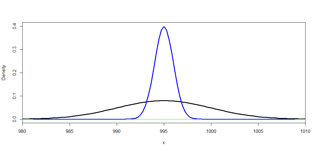
Addendum: In the figure below, the black curve is the density curve for the population of weight measurements,
which is $\mathsf{Norm}(\mu = 995, \sigma = 5).$ That
determines the variability of individual measurements $X_i.$
The blue curve is the density curve for $\bar X,$ means of samples of size $n=25.$ Its standard deviation is $\sigma_{\bar X} = \sigma/\sqrt{n} = 5/\sqrt{25} = 1.$ This curve governs the margin of error of a 95% CI based on 25 observations.
It is one fifth as 'wide' as the population density and so five times as 'tall'. Both curves enclose a total probability of $1.$


