Historically, did pseudo RNGs have range [0,1] because of the ease of drawing from $f$ using $F^{-1}(p)$, or for some other reason?

Question

A simple, though not necessarily efficient, way to simulate random draws from a probability density function $f$, is to apply the inverse cumulative distribution function to a random variate distributed uniformly from 0 to 1. The pseudo random number generators (RNGs) I am (barely) familiar with produce pseudo-random values having this kind of distribution.

I do not really know much about the history of how RNGs were developed, but I wonder if RNG default behavior was expressly designed because of its suitability for simulating from arbitrary distributions (or at least from arbitrary distributions with computable inverse cumulative distribution functions)? Or are there other reasons why RNG algorithm output should range [0,1]—as opposed to [-1, 1], [0, floating point limit], or [0, long limit], etc.—and specifically with a uniform, as opposed to some other distribution?

I know that, statistical properties aside, computational algorithms have other properties, e.g., security, memory use, computational complexity, etc., which weigh on development and adoption of a RNG algorithm; any insights welcome.

Answer 1

In principle, any continuous distribution can serve as a starting point for a random number generator. Nevertheless, the standard continuous uniform distribution is a natural starting place for a pseudo-random number generator (PRNG) for a few main reasons:

• The method of inverse transformation sampling allows us to generate any random variable from a standard uniform random variable, and the latter is a natural starting place for this computation. In particular, the mathematics of transforming a standard uniform random variable to a random variable with another distribution is particularly simple and intuitive.

• The standard uniform distribution has particularly simple properties for the purposes of testing the accuracy of the PRNG method. These methods are subject to a battery of tests to ensure that they have desirable properties for a random number generator. These tests are particularly easy to frame for a PRNG that generates a standard continuous uniform random variable. For example, standard occupancy tests are particularly easy to deploy for uniform random variables.

• Computational methods that generate real numbers are subject to rounding error. In most platforms the numbers are stored in double-precision floating point format, and this format has a fixed level of accuracy in the fractional part. When generating a standard continuous uniform random variable the interval between values of the fractional part have fixed probability, so no intervals are larger or smaller than others. (Contra this reasoning, note that this is also arguably a reason to prefer an exponential random variable as the starting point for analysis, since the floating point format uses an exponent.)

Answer 2

Vetting a PRNG. First, the standard uniform distribution $\mathsf{Unif}(0,1)$ is mathematically simple. So given pseudorandom numbers that are purported to be indistiguishable, for practical purposes, from a random sample from a standard uniform population, it is easy to test whether the claim is true.

For example, close to $1/10$th of the observations should lie in each of the intervals $(0.1k, 0.1k+.1),$ for $k = 0, \dots, 9,$ and we can do a chi-squared goodness of fit test to see if that is true.

Today in R, the procedure runif(10^4) generates $10\,000$ observations supposedly from $\mathsf{Unif}(0,1).$

set.seed(510)
u = runif(10^4)
hist(u, br=seq(0,1,by=.1), ylim=c(0,1200), label=T)

x = hist(u, br=seq(0,1,by=.1), plot=F)$counts; x
[1]  959  960 1044 1048  966 1001 1044 1001  990  987

So we see that the $10\,000$ observations are consistent with a sample from $\mathsf{Unif}(0,1).$ [In chisq.test equal probabilities for groups are assumed if no other probabilities are supplied.]

chisq.test(x)

        Chi-squared test for given probabilities

data:  x
X-squared = 10.884, df = 9, p-value = 0.2837

    Chi-squared test for given probabilities

data:  x
X-squared = 10.884, df = 9, p-value = 0.2837

And so on, through many more tests to vet the random number generator as useful.

Quantile method for continuous distributions. Second, as you say, it is possible to use the quantile (inverse CDF) transform to get samples from a vast variety of other distributions. So that the transform below should give us a pseudo-random sample from $\mathsf{Exp}(1).$

w = qexp(runif(10^5), 1)
hist(w, prob=T, br=50, col="skyblue2")
 curve(dexp(x,1), add=T, col="red", n=10001)

In the figure above, a standard uniform density curve seems a good fit to a density histogram of the data. Also, a Kolmogorov-Smirnov test does not reject the null hypothesis that the first 5000 values in w are a sample from a standard uniform distribution. [The test does not allow samples larger than 5000.]

ks.test(w[1:5000], pexp, 1)

        One-sample Kolmogorov-Smirnov test

data:  w[1:5000]
D = 0.0054447, p-value = 0.9984
alternative hypothesis: two-sided

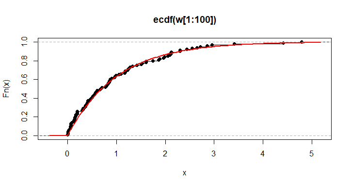
The test statistic $D$ of the K-S test is the maximum vertical discrepancy between the target CDF and the empirical CDF of the sample (a stairstep function of sample values that approximates the CDF). We illustrate with a sample of size 100.

ks.test(w[1:100], pexp, 1)

        One-sample Kolmogorov-Smirnov test

data:  w[1:100]
D = 0.076693, p-value = 0.5988
alternative hypothesis: two-sided

plot(ecdf(w[1:100]))
curve(pexp(x,1), add=T, col="red", lwd=2)

Quantile method for discrete distributions. The quantile transform method also works for discrete random variables (provided that the quantile function is carefully programmed, as it is in R). So let's simulate a sample from $\mathsf{Binom}(10, .5):$ [The R procedure ks.test does not apply to discrete distriubtions.]

v = qbinom(runif(5000), 10, .5)
hist(v, prob=T, br = (-1:10)+.5, col="skyblue2")
  vv = 0:10;  pdf = dbinom(vv, 10, .5)
  points(vv, pdf, col="red")

Notes: (1) In R, the quantile method us used to generate normal random samples—even though the normal CDF cannot be expressed in closed form and thus cannot be inverted analytically. R uses Michael Wichura's (piecewise) rational approximation to the standard normal CDF, and his inversion of it. Results are accurate up to double-precision arithmetic.

set.seed(2020);  rnorm(1)
[1] 0.3769721
set.seed(2020);  qnorm(runif(1))
[1] 0.3769721

Earlier methods of simulating standard normal variates were (a) to use $\sum_{i=1}^2 U_i - 6,$ where $U_i \stackrel{iid}{\sim} \mathsf{Unif}(0,1),$ which relies on the quick convergence of the CLT for uniform random variables and requires only simple arithmetic operations, and (b) to use the Box-Muller transformation, which is somewhat more accurate and requires computing logarithmic and trigonometric functions.

(2) Undoubtely, there are many other reasons: some of them lost history from the mid-1950s, and some possibly yet to come here in additional answers or comments.