Random number (between 0 & 1; > 5 decimal places) from binomial/beta-like distribution, with set mean (same as mode & median) and set variance

Question

Due to misunderstandings and as per request I have rollbacked this question to this previous state. Please do not answer this question instead answer this one: Random number (between 0 & 1; > 5 decimal places) from skewed binomial/beta-like distribution, with set mean (same as mode) and set variance

First of all this question is very similar/the same as others linked just below. However, none of the answers I saw are correct/precise enough for a distribution with the same mean, mode and median.

Distribution that has a range from 0 to 1 and with peak between them? & Beta-distribution: how to generate a peak at certain mean value with a control on variance in extrems

I first tried binomial, as it didnt work out I tried the beta-distibution people suggested on the other answers. tl;dr: Binomial has the same mean, mode and median, but the number of decimal places are dependent on variance so I cannot choose it freely. Beta distribution allows me to choose variance and has enough decimal places but mean, mode and median are not the same.

Here are the rules the random number X needs to follow:

Conditions that X itself has to fulfill:

1. X must be between 0 to 1 (including 0 and 1).
2. X must have at least 5 decimal places. (ideally unlimited, but 5 would be enough maybe even 4)

Conditions that the probability density function (pdf) from which X is drawn hast to fulfill

1. The mean is also the modus/maximum and median if possible.
2. The pdf should look like a binomial distribution.

Input that I give:

1. The mean. (which should also be the most likely number to be drawn and be the median).
2. I want to be able to change the variance freely, but relative to the mean (e.g. if mean is 0.6 variance should be 0.2 but if mean is 0.99 variance shouldnt be 0.2).

I have not managed to either get binomial distributions nor beta distributions to work. I haven't found anything else. Here is the problems with either distributions.

Problem with the binomial distribution:

I cannot set the variance independently from the number of decimal places. E.g. if I want to have high variance I can do that by reducing the amount of events I simulate in the binomial distribution. For example only 6, however that means that I reduce my possible numbers to (0,0.2,0.4,0.6,0.8,1). If I increase the events then I get more decimal places however the pdf will be extremely narrow around the mean.

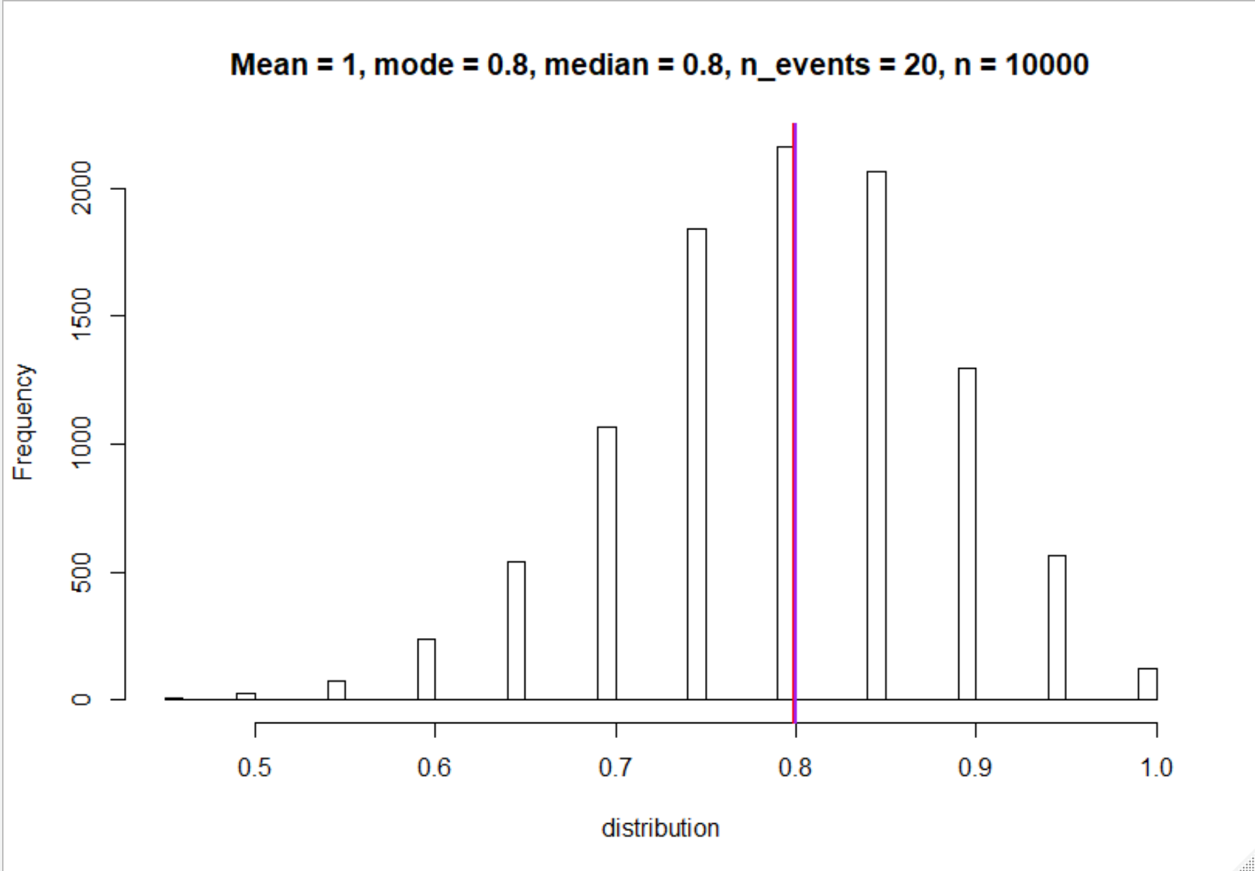
Histogram with events = 5, n =100,000, mean 0.8. Good variance, but numbers dont have enough decimal places. Mean (red),mode/maximum (blue), median (purple), cant be seen cause they overlap.

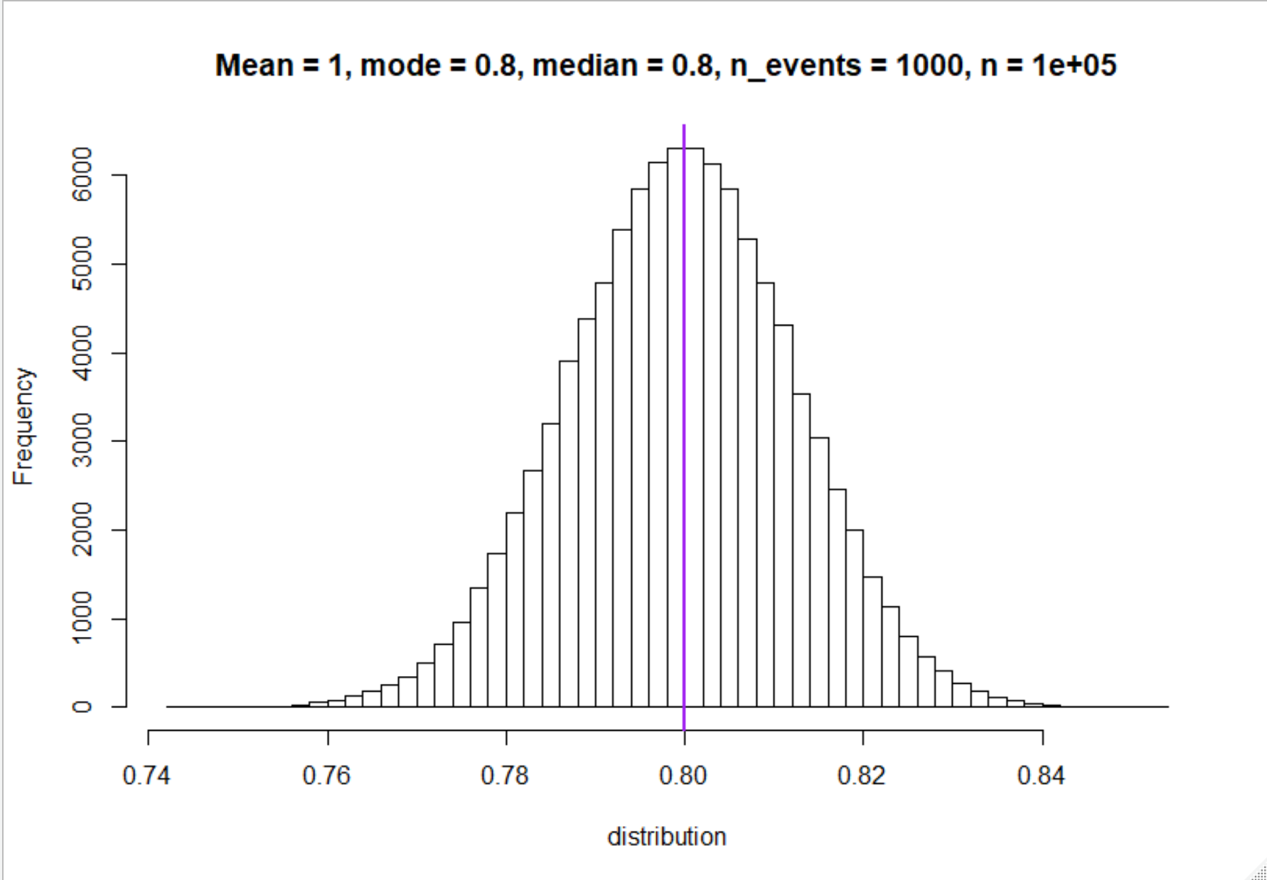
Histogram with events = 1000, n =100,000, mean 0.8. Too little variance, see x axis units.

Code for binomial distribution (in R):

#Binomial Distribution
n_events<-10 #e.g. 10 coinflips 
probability<-0.8 #with an 80% chance of success
numbers_drawn<-100000 #how many times you do the same experiment e.g. throw 10 coins 100000 times
distribution<-rbinom(numbers_drawn, n_events, probability)/n_events #divided by n_events to rescale numbers between 0 and 1
#print(distribution)
#events = 5, 10 numbers_drawn: 1.0 0.7 0.9 0.9 0.9 0.9 0.8 0.8 0.7 1.0
#events = 1000 , 10 numbers_drawn: 0.773 0.801 0.811 0.798 0.792 0.783 0.797 0.802 0.771 0.803

#calculate mode (no R function in base package)
dist<-round(distribution, digits = 3) #if you set really narrow pdfs you  need to round to more digits to get an accurate mode
uniqv <- unique(dist) #groups same numbers
mode<-uniqv[which.max(tabulate(match(dist, uniqv)))] #which number occurs most often

hist(distribution, breaks = 40, main = paste0("Mean = ", round(mean(distribution)),", mode = ", mode,", median = ", median(distribution), ", n_events = ", n_events , ", n = ", numbers_drawn))
abline(v = c(mean(distribution), mode, median(distribution) ), col = c("red", "blue", "purple"), lwd = 2)   #plot vertical lines
print(c(mean(distribution), mode, median(distribution)))

Problem with beta distribution:

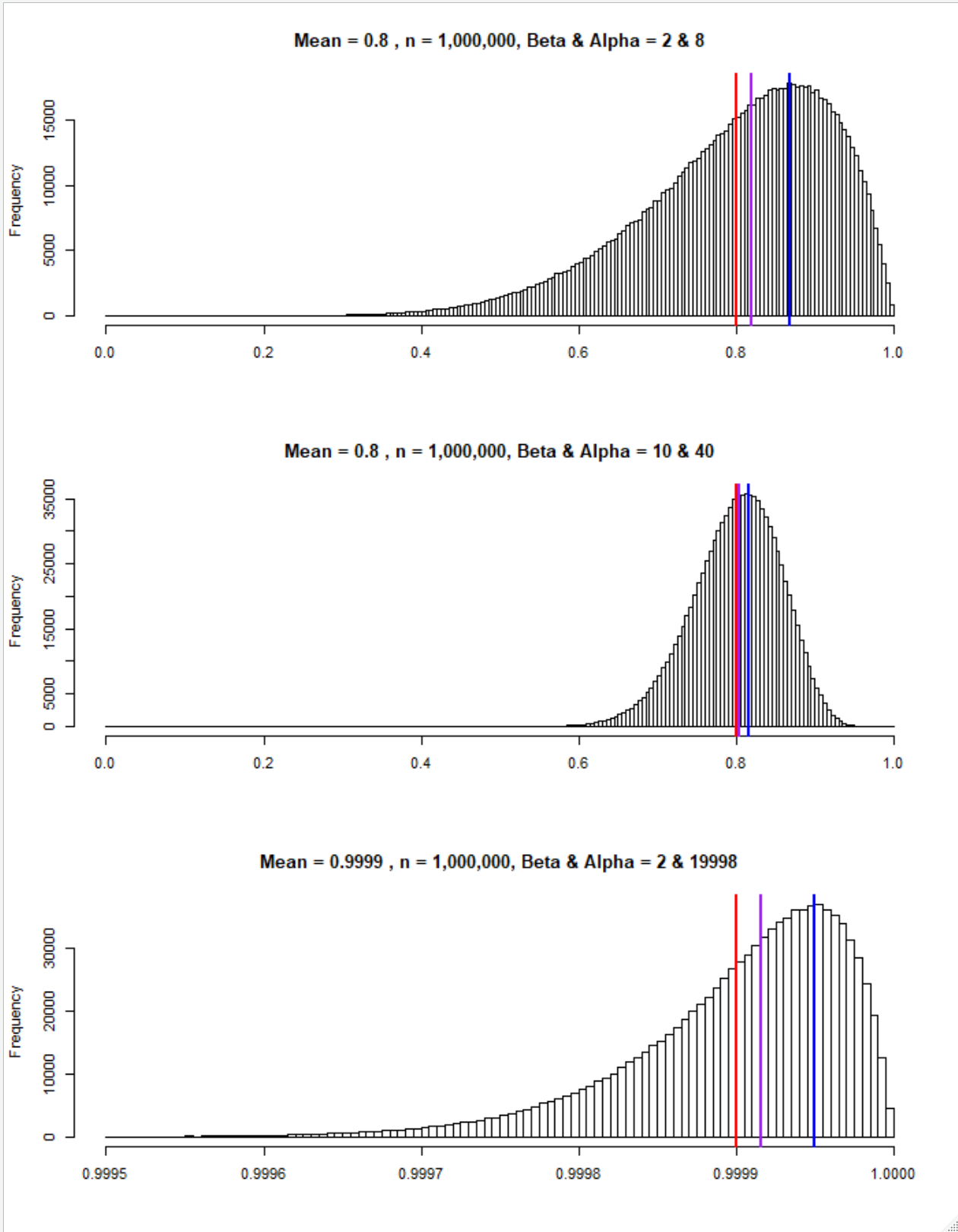
The beta distribution allows me to keep variance the same (relatively to the Mean) but change the Mean freely. I have accomplished this by keeping beta always at a certain number and varying alpha, based on the mean (see the code). At first glance it looks right but unfortunately the mean (red) does not coincide with the mode/maximum (blue) nor median (purple).

Mean (red),mode/maximum (blue), median (purple) Now I can correctly set variance however I want, but the median and mode are higher than the mean. Because someone on one of the linked questions a the top thought this couldnt work; I added the last plot to showcase that this works for any mean. It works because as long as alpha and beta are above 1. As alpha is always higher than the set beta there are no weird edge cases.

Do you have any ideas on how to have a distribution like the binomial one (first pic) but with more decimal places. Is this even possible? Even if I can already have the same mean and mode or same mean and median it would already be great.

Code for Beta Distribution (in R):

   mirror<-FALSE # mirror the distribution
  #if mean > 0.5 beta should be the smaller number. else alpha should be the smaller
  #if one exchanges alpha and beta distribution is mirrored
  #it is easier to mirror it than recalculating alpha if beta is set
  mean_original<-0.8
  mean<-mean_original
  if (mean < 0.5) { 
    mirror<-TRUE 
    mean<-1-mean 
  }
  beta<-10       #if you set beta higher it will narrow the pdf; below 1.5 it might lead to unintuitive output with maximum being super close to 1 or 0
  alpha<- (-beta*mean)/(mean-1)    #calculate mean solved for alpha
  var<-(alpha*beta)/((alpha+beta)^2*(alpha+beta+1)) #standard variance calculation
  #var<-(mean^3-2*mean^2+mean)/(beta-mean+1)  #calculate var just from beta and mean
  #alpha <- ((1 - mean) / var - 1 / mean) * mean ^ 2   #calculate alpha from variance and mean
  if (mirror) {
    distribution<-stats::rbeta(1000000, beta, alpha, ncp = 0) #mirror the distribution 
  }else{
    distribution<-stats::rbeta(1000000, alpha, beta, ncp = 0) #ncp = non-centrality parameter 0 is default
  }
  #if you want the mode/maximum to be e.g. 0.8, set mean to 0.8 and add 1 each to alpha and beta, however your mean is not gonna be 0.8 anymore
  print(mean(distribution)) # check if mean is what it should be
  
  #calculate mode (most common number/maximum of the pdf)
  dist<-round(distribution, digits = 5) #if you set really narrow pdfs you  need to round to more digits to get an accurate mode
  uniqv <- unique(dist) #groups same numbers
  mode<-uniqv[which.max(tabulate(match(dist, uniqv)))] #which number occurs most often
  print(mode)
  cutoff<-0 #allows you to cuttoff for plotting purposes (to "zoom in" to a specific area) 
  hist(subset(distribution, distribution > cutoff),breaks = seq(cutoff,1,0.005), main = paste("Mean =", mean_original, ", n = 1,000,000, Beta & Alpha =", beta, "&", round(alpha)), xlab = "")
  abline(v = c(mean(distribution), mode, median(distribution) ), col = c("red", "blue", "purple"), lwd = 2)   #plot vertical lines

Answer 1

It sounds like you are asking for a scaled version of a Beta variable:

• For the median to equal the mode, the two Beta parameters must be equal.
• For the distribution to be symmetric, the two Beta parameters must be equal.
• For it to have just one central mode, the common Beta parameter must exceed $1.$
• For its values to be supported in the interval $[0,1],$ the scale factor cannot exceed one-half the smallest of $\mu$ and $1-\mu.$ Let the actual scale factor be $f$ times this limiting value, with $0\lt f \le 1.$

For a given target mean/mode $\mu$ and relative scale factor $f$ set $s(\mu, f) = f\min(\mu,1-\mu).$ Then for a variance of $v$ the Beta parameter must exceed

$$\alpha(\mu,\sigma,f) = \frac{1}{2}\left(\frac{s(\mu, f)^2}{v}-1\right).$$

Shift and scale this Beta variable to place its mean (which is $1/2$) at $\mu$ and to give it the desired variance. Here is an R implementation to generate $n$ independent draws from this distribution:

rf <- function(n, mu, v, f=1) {
  if (isTRUE(mu <= 0 | mu >= 1)) stop("Invalid mean.")
  if (isTRUE(f > 1)) stop("Invalid scale factor.")
  s <- min(mu, 1-mu) * f
  alpha <- (s^2/v - 1)/2 
  if (isTRUE(alpha <= 0)) stop("Variance too large.")
  ((2*s) * rbeta(n, alpha, alpha) - s) + mu
}

Its values are double-precision floats, giving over 15 decimal digits of precision.

The figure shows histograms of one million draws (each) from five such distributions. Following it is the R code showing how rf was used to create the figure.

Notice how, in the left examples (with the same mean and variance), scaling the distribution down forces the Beta parameter to be smaller, changing the distributional shape. I introduced the parameter $f$ expressly to create this flexibility.

parameters <- list(
  c(mu=0.5, v=1/50, f=1),
  c(mu=0.5, v=1/50, f=1/2),
  c(mu=0.8, v=0.004, f=1),
  c(mu=0.1, v=0.001, f=3/4),
  c(mu=1/3, v=0.005, f=1)
)
n <- 1e6
par(mfrow=c(1, length(parameters)))
for(i in seq_along(parameters)) {
  p <- parameters[[i]]
  x <- rf(n, p["mu"], p["v"], p["f"])
  mu.s <- sprintf("%.2g", p["mu"])
  v.s <- sprintf("%.2g", p["v"])
  f.s <- sprintf("%.2g", p["f"])
  hist(x, freq=FALSE, breaks=50, xlim=0:1, 
       border="#00000040", lwd=0.1, col=hsv(i/length(parameters), .65, 1),
       main=bquote(paste(mu==.(mu.s), ", ", sigma^2 == .(v.s), ", and ", f == .(f.s))))
  abline(v = mean(x))
}

Answer 2

This is a reply to a question asked by the OP in comments [edited for grammar]:

Can you explain what kind of binomial distributions does not have mean, median and mode equal? All the ones I plotted had that property.

This won't go easily as a comment. It's an example of a binomial in which the mean, median and mode do not all coincide. The table shows probabilities for (0, ..., 10) successes out of 10 if probability of success is 0.05. The median and mode are both 0 but the mean isn't. The syntax is Stata syntax but the calculation is, or should be, standard in any good software. There are many other such examples.

Another way to see this is that the median and mode must be an integer or conventionally a half-integer if adjacent values have equal frequencies, but there is no such rule for the mean.

. mata : (0::10), binomialp(10, (0::10), 0.05)
                  1             2
     +-----------------------------+
   1 |            0   .5987369392  |
   2 |            1   .3151247049  |
   3 |            2   .0746347985  |
   4 |            3   .0104750594  |
   5 |            4   .0009648081  |
   6 |            5   .0000609352  |
   7 |            6   2.67260e-06  |
   8 |            7   8.03789e-08  |
   9 |            8   1.58643e-09  |
  10 |            9   1.85547e-11  |
  11 |           10   9.76563e-14  |
     +-----------------------------+