Fixed vs Random
I know this is an old question but I don't believe the old answer here really tackles the question fully. There are three ways you can think about it: what I will informally call the theoretical perspective, the data reduction perspective, and the replication perspective.
The theoretical perspective is that the fixed effects are those that you are actually interested in modeling as a direct effect on your outcome variable. We could include someone's gender/sex as a categorical predictor of income because we know from past research that these variables have some relationship with each other and can be an important one to investigate. However, some would be less concerned with, for example, the neighborhood someone comes from with relation to income if its not important to their model (though certainly this doesn't mean other researchers wouldn't find it so). If included as a random effect, we are in some part implying that we just think it's an annoyance factor that needs to be removed to clean up how accurate our fixed estimates are (though see below for when thats not such the case). A key thing to notice here is that one person's fixed effect can be another person's random effect depending on what they're trying to say about their model.
Another perspective, one that I think is often lost when mixed models are taught, is the data reduction perspective, which is simply that we want to summarize a lot of information about variations in a DV based off selected clusters. This in my opinion is often more informative, because we often aren't interested in a random effect with few levels or one that doesn't include a lot of variance...we want something normally that varies a lot in order to 1) summarize the average distance from, say, the conditional mean 2) specifically compare across a variety of clusters (for example seeing which schools are above the mean in reading outcomes over others) and 3) remove bias from standard errors in the regression. On a separate note, it also greatly reduces down the amount of information one has to interpret from the fixed effects portion of the model. Typically when you have a standard regression that uses a categorical variable with many levels, you will get as many coefficients as there are levels. This consequently can be a bit confusing to digest.
Whereas many regressions are less concerned with what the random noise is trying to tell us, mixed models operationally add it in to inform researchers about a large depth in heterogeneity across settings, people, or other contextual factors so that we have more accurate assumptions about what the fixed effects are actually doing. This "pollution" in random variance can actually tell us a lot. A great example is the classic subject x item crossed effects design, wherein we can learn a lot about the ease/difficulty of different items and subject aptitude in general while untethering it from what fixed effects we deem important. These first two perspectives are already both important for selecting a categorical effect as either fixed or random. How one selects them is heavily weighted by theory as well as the underlying data supporting such models.
Having said that, there is another way to look at this that I believe helps solidify the distinction more, and that is the importance of the replication perspective. When we consider fixed effects, we are interpreting the effects as those we should see across studies with some semblance of stability. In other words, these are population-level effects that we are trying to infer from the model. With repeated experiments, our understanding of the fixed effects should converge into an average effect of interest. This is not the case for random effects, where by definition we consider these effects to be totally random and should not have a predictable pattern (other than average variance perhaps). These are more sample-level effects that we want to untangle because they muddy the waters with respect to the population-level effects.
As an example from Simon Wood's book on GAMs (p.72), the chapter on mixed models provides this example:
Now consider a practical example. The Machines data frame, from the
nlme package, contains data from an industrial experiment comparing 3
different machine types. The aim of the experiment was to determine
which machine type resulted in highest worker productivity. 6 workers
were randomly selected to take part in the trial, with each worker
operating each machine 3 times (presumably after an appropriate period
of training designed to eliminate any ‘learning effect’)...
We are interested in the effects of these particular machine types, but are only interested in the worker effects in as much as they reflect variability between workers in the population of workers using this type of machine. Put another way, if the experiment were repeated somewhere else (with different workers) we would expect the estimates of the machine effects to be quite close to the results obtained from the current experiment, while the individual worker effects would be quite different (although with similar variability, we hope).
This should further clarify the difference between fixed and random effects, as it should be clear that with your example, classes should not have a predictable fixed effect on the outcome given how widely they would vary from experiment to experiment.
Why This Matters for Your Comparison
Recall that above I mentioned how random effects influence the standard errors. This is because typically regressions which do not account for correlated errors are downward biased...in other words they greatly underestimate how influential an actual effect is because the accuracy of these estimates is influenced by the clusters in the data.
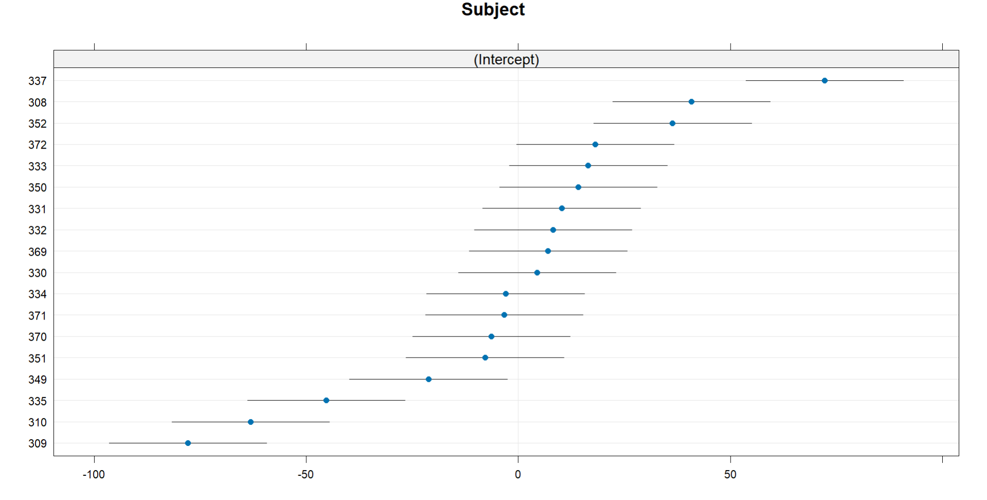
Probably the biggest reason you aren't seeing the big picture is because you are only looking at point estimates for the fixed effects in each regression. I fit a common toy dataset in R called sleepstudy to a lmer model below, then summarize and plot the random effects.
#### Load Libraries ####
library(lmerTest)
library(lattice)

#### Fit Data ####
fit <- lmer(Reaction ~ Days + (1|Subject),
            data = sleepstudy)
summary(fit)

#### Plot ####
dotplot(ranef(fit))
The summary is quite long, but the part you probably skipped is this portion that follows, which shows how the random effects vary (here subjects vary in reaction time substantially). This means that the day of this study effected reaction time, but this varied by subject, and without modeling this we cost ourselves some accuracy in the estimated effect consecutive day has on reaction time.
Random effects:
 Groups   Name        Variance Std.Dev.
 Subject  (Intercept) 1378.2   37.12
 Residual              960.5   30.99
Number of obs: 180, groups:  Subject, 18
Plotting the random effects shows a great summary of the random effects, which show by-subject variance around the conditional mean, the points being the average effect and the bars around it the fluctuation around those means. For example, Subject 337's reaction time is far slower on average, whereas Subject 309 is quite quick compared to others.

Going back to my previous point, this is important, as we could have just as easily entered Subject in as a fixed effect. However, this would have given us a ton of coefficients (one per subject), now way to meaningfully summarize their differences, and likely wouldn't be theoretically meaningful.

