If a likelihood function can take any shape, how can we trust the score test?

Question

I am under the impression (perhaps wrongly) that a likelihood function can, theoretically, take on any shape (depending on observed data and the parameters being estimated). Below is an example of a log likelihood function. On the y-axis is log likelihood of the observed data given some parameter value and the x-axis is the parameter values.

In this case, the log likelihood function is a lovely parabola. So as you move further away from the maximum likelihood estimate, at which the score (gradient) is 0, the gradient of the function becomes more and more steep (i.e. the score increases). This, in turn, increases the test statistic of a score test, $Q$:

$Q = \frac{score(\beta_{null})^2}{var(\beta_{null})}$

This makes sense to me. The parameter estimate under the null hypothesis is "far" from the MLE of the parameter, hence high test statistic, low p-value, reject null hypothesis.

What happens then if the log likelihood function isn't a parabola? What if say, it happened to look like this:

Notice how the score (gradient) of the function begins to decrease again at the tails. This would begin to make the test statistic smaller, increasing the p-value, making it appear as if we should be accepting the null hypothesis. When in reality, the MLE is far away from the parameter value assuming the null hypothesis.

Answer 1

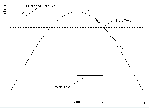
"When in reality, the MLE is far away from the parameter value assuming the null hypothesis"—if distance of the maximum-likelihood estimate from the null is your measure of discrepancy with the null then you can use it as your test statistic. The point of the score test is to maximize power against alternatives close to the null (when the M.L.E oughtn't to be too far away).^†

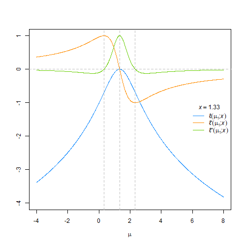
Consider, say, a single observation $x$ from a Cauchy distribution with unknown location parameter.The log likelihood, score, & the 2nd derivative of the log likelihood are given by $$ \begin{align} \ell(\mu;x) &= -\log(1+(x-\mu)^2)\\ \frac{\operatorname{d}\ell(\mu;x)}{\operatorname{d}\mu} &= \frac{2(x-\mu)}{1+(x-\mu)^2}\\ \frac{\operatorname{d}^2\ell(\mu;x)}{(\operatorname{d}\mu)^2} &= \frac{1}{1+(x-\mu)^2} - \frac{2(x-\mu)^2}{(1+(x-\mu)^2)^2}\\ &=\frac{1-(x-\mu)^2}{(1+(x-\mu)^2)^2} \end{align} $$

The M.L.E. is obviously given by $\hat\mu=x$; note also the inflection points in the log likelihood at $x\pm 1$ & the corresponding minimum & maximum of the score.

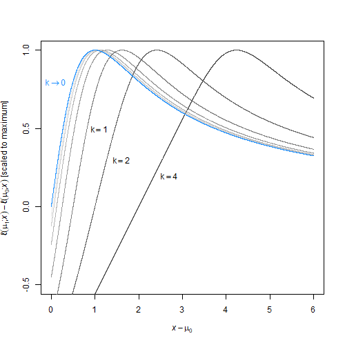
For a test of $H_0: \mu = \mu_0$ vs $H_1: \mu = \mu_1 = \mu_0 + k, k>0$, as any observation $x\gg k$ is only marginally more probable under the null than the alternative, the log likelihood ratio $\ell(\mu_1;x) - \ell(\mu_0;x)$ as a function of $x$ increases to a maximum^‡ & then decreases asymptotically to zero. But as $k\rightarrow 0$ a limit is approached, proportional to the score.

Therefore there's no uniformly most powerful test of $H_0: \mu = \mu_0$ vs $H_1: \mu > \mu_0$, & a locally most-powerful test might be what's wanted—trading off power against distant alternatives for power against near ones. (Or if not, the generalized likelihood test statistic $\ell(\hat\mu;x)- \ell(\mu_0;x)$ is a monotonic function of $x$ for $\hat\mu>\mu_0$.)

In other cases, say i.i.d. observations following a Poisson distribution, the score & generalized likelihood ratio will order the sufficient statistic identically (for one sided tests at any rate), so the exact tests will be equivalent. If you're relying on an asymptotic approximation to the distribution then you'll get somewhat different results with the two as kjetil's answer points out.

---

† By the Neyman–Pearson Lemma, the most powerful test of a point null $H_0: \theta= \theta_0$ against a point alternative $H_1: \theta= \theta_0 + \delta$ is given by the log likelihood ratio

$$\ell(\theta_0 +\delta;x) - \ell(\theta_0;x)$$

A Taylor expansion of the log likelihood under the alternative around $\theta_0$ gives

$$\ell(\theta_0 +\delta;x) \approx \ell(\theta_0;x) + \delta \cdot\left.\frac{\operatorname{d}\ell(\theta;x)}{\operatorname{d}\theta}\right|_{\theta=\theta_0}$$

& so for small $\delta$ the log likelihood ratio becomes proportional to the score.

‡ A root of $x^2 - (\mu_0 + \mu_1)x + (\mu_0 \mu_1 - 1)$.

Answer 2

Your question is very general, and I think the answer is that, in general, there is no reason to think the score test is good. In the parabolic test you have shown, the score test is equivalent to the likelihood ratio test, which is often considered as "gold standard". If the likelihood function is far from quadratic, the score test might not be dependable.

In situations where the usual asymptotics is valid (that is, with a normal/Gaussian limit distribution), these are asymptotically equivalent, so with large enough sample sizes, the score test should work.

But, a full answer in this generality is not possible, it must be investigated for specific models.