Should I use a one-sided or a two-sided test when deciding to deploy new system? [duplicate]

Question

In the following situation, should I use a one-sided or a two-sided significance test?

Situation: Suppose I have a face recognition system A that recognizes faces with a certain accuracy. Now I want to test if my new system B has significantly better accuracy. If it does, I will deploy B. If B is just the same or even worse than A then I will not deploy B.

Related question: I have a related question about two-sided tests, specifically: Rejecting the null hypothesis here would mean that the new system B different from A, which means it could be significantly worse or significantly better -- the two-sided test does not say which it is. Correct? If that's correct, what could be the value of a two-sided test in my situation above, where I want to avoid deploying a system that is worse than the existing system?

Answer 1

I think this is actually a perfect use of a one-tailed test. The risk of one-tailed tests is the potential to capitalize on chance, but this is not an issue here since you have explicitly defined the important region of the parameter space a priori, and done so in a practically justified way. As long as you truly take no new action as a result of a large effect in the opposite direction, there seems to be nothing wrong with a one-tailed test in this instance.

The p-value of a two-sided test doesn't tell you the direction of the effect, but the effect estimate does. If the mean for B is greater than the mean for A and the two-sided p-value is small enough to reject the null hypothesis that the true means are the same, then you can say that the true mean for B is greater than the true mean for A, the same conclusion you would reach with a significant one-sided test in the right direction.

Answer 2

Thanks for the careful explanation of your question. You do need a one-sided test.

If you happen to have computer output for a two-sided test and the sample means are in the proper relationship, you can conclude that a one-sided test will have half the P-value of the two-sided test.

Fictitious data for illustration (sampled using R):

set.seed(2021)
x.a = rnorm(70, 50, 4)
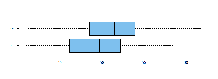
summary(x.a)
   Min. 1st Qu.  Median    Mean 3rd Qu.    Max. 
  40.98   46.18   49.76   49.64   52.16   58.48 
x.b = rnorm(70, 52, 4)
summary(x.b)
   Min. 1st Qu.  Median    Mean 3rd Qu.    Max. 
  41.20   48.75   51.46   51.22   53.94   61.81 

boxplot(x.a, x.b, col="skyblue2", horizontal=T)

Two-sided test: $H_0: \mu_a = \mu_b$ against $H_a: \mu_a \ne \mu_b.$ Reject with P-value $0.03 < 0.05 = 5\%.$

t.test(x.a, x.b)

        Welch Two Sample t-test

data:  x.a and x.b
t = -2.2045, df = 137.96, p-value = 0.02915
alternative hypothesis: true difference in means is not equal to 0
95 percent confidence interval:
 -3.0078510 -0.1633819
sample estimates:
mean of x mean of y 
 49.63691  51.22252 

The P-value can be found in R, where pt is the CDF of Student's t distribution. The Welch test can use fractional degrees of freedom, which some software rounds to integers.

L = pt(-2.2045, 137.96)    # actual left tail probability
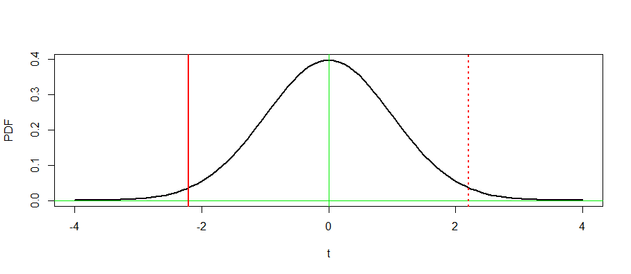
R = 1-pt(2.2045, 137.96)   # just as extreme in right tail
L+R
[1] 0.02914627

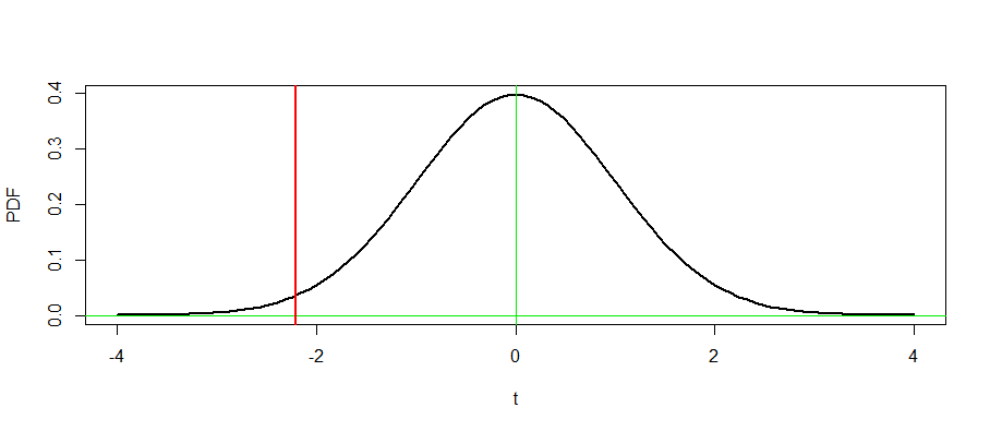
In the figure bwlow, the P-value is the sum of the areas under the density curve in the two tails beyond the vertical red lines.

curve(dt(x,127.96), -4, 4, ylab="PDF", xlab="t", lwd=2)
 abline(h=0, col="green2");  abline(v=0, col="green2")
 abline(v =-2.2045, col="red", lwd=2)
 abline(v = 2.2045, col="red", lwd=2, lty="dotted") 

One-sided test: $H_0: \mu_a \ge \mu_b$ against $H_a: \mu_a < \mu_b.$ Reject with P-value $0.015 < 0.02 = 2\%.$

t.test(x.a, x.b, alt="less")

        Welch Two Sample t-test

data:  x.a and x.b
t = -2.2045, df = 137.96, p-value = 0.01457
alternative hypothesis: true difference in means is less than 0
95 percent confidence interval:
       -Inf -0.3945112
sample estimates:
mean of x mean of y 
 49.63691  51.22252 

The P-value is found as follows, using R.

pt(-2.2045, 137.96)
[1] 0.01457313