If $20 $ random numbers are selected independently from the interval $(0,1) $ probability that the sum of these numbers is at least $8$? [closed]

Question

If $20 $ random numbers are selected independently from the interval $(0,1) $ what is the probability that the sum of these numbers is at least $8$?

I tried to take this question https://math.stackexchange.com/questions/285362/choosing-two-random-numbers-in-0-1-what-is-the-probability-that-sum-of-them as reference but the step where there is a double integral, I got stuck, do I have to make 20 integrals?

Answer 1

It can be helpful to have a "gross reality check" (or grc) ((some people call it a sanity check)) that comes at the problem side-ways and can tell you if you are doing something wrong.

Here is R-code to simulate the problem, and give an estimate:

set.seed(1)
  temp <- numeric(length=20000)
  for(i in 1:20000){
    # y <- sample(c(0,1),20,T)   # (wrong! Thanks @whuber) discrete
    y <- runif(n=20)  # continuous outputs
    
    # is it 8 or more
    temp[i] <- ifelse(sum(y) >= 8, 1, 0)
  }
  mean(temp)

This is what it gives:

> mean(temp)
[1] 0.94265

After 20k trials I would expect the estimate to be within 1% or 0.1% of theoretical result.

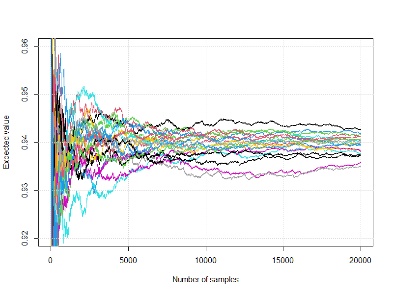
Here is a plot of 20 runs, showing convergence and spread of the estimate

Here is the list of the tail value for the runs, and the residual from the ensemble mean:

          mean      err
    1  0.94265  0.00324
    2  0.94160  0.00219
    3  0.93955  0.00014
    4  0.94190  0.00249
    5  0.93775 -0.00166
    6  0.93580 -0.00361
    7  0.93840 -0.00101
    8  0.93500 -0.00441
    9  0.93735 -0.00206
    10 0.94030  0.00089
    11 0.94160  0.00219
    12 0.93965  0.00024
    13 0.94005  0.00064
    14 0.93810 -0.00131
    15 0.93990  0.00049
    16 0.93995  0.00054
    17 0.93735 -0.00206
    18 0.94125  0.00184
    19 0.94070  0.00129
    20 0.93935 -0.00006

They don't move around much. The standard deviation in those means is ~0.00204, while the ensemble mean is 93.941%

The estimates 93.94% (analytic) and 93.941% (simulated) are ~0.0048 standard deviations apart, which indicates to me that the analytic approach is on the right track.

Answer 2

Let $ \ X_i $ be the $ \ i^{th}$ number selected where $\ i= 1,2,3,4...20 $

$To $ $ calculate $

$ \ P( \sum_{i=1}^{20} X_i \ge 8 ) $

$ E(\ X_i) = \frac{(0+1)}{2} $ $ [uniform $ $ distribution ] $

$ E(\ X_i) = \frac{1}{2} $

$ E(\sum_{i=1}^{20} X_i) = 20/2 = 10 $

$ Var(\ X_i) = \frac{\ (1-0)^2}{12} $ $ [uniform $ $ distribution ] $

$ Var(\ X_i) = \frac{\ 1}{12} $

$ Var(\sum_{i=1}^{20} X_i) = 20/12 = 5/3 $

$ \ P(\frac{ \sum_{i=1}^{20} X_i - E(\sum_{i=1}^{20} X_i) }{\sqrt Var(\sum_{i=1}^{20} X_i)} \ge \frac {8 -E(\sum_{i=1}^{20} X_i)}{\sqrt Var(\sum_{i=1}^{20} X_i} ) $

$ \ P(\frac{ \sum_{i=1}^{20} X_i - 10) }{\sqrt {5/3}} \ge \frac {8 -10}{\sqrt 5/3} ) $

$ 1- P(Z \le -1.55)$

= $ 0.9394 $ $ approx $

Answer 3

Here is a histogram of 100,000 simulations each taking the sum of 20 uniform random deviates. Based on this simulation the sum of uniform deviates is well approximated by a normal distribution with an estimated mean of 10.004 and an estimated variance of 1.680. Using the normal approximation the probability that $\sum_{i=1}^n X_i \ge 8$ is $0.94$.

Code follows:

data uniform;
  do sim=1 to 100000;
    do i=1 to 20;
        y=rand('uniform');
        output;
    end;
end;
run;

proc means data=uniform noprint;
by sim;
var y;
output out=out sum(y)=sum;
run;


ods graphics / height=3in width=6in border=no;

proc sgplot data=out;
histogram sum;
density sum / type=normal;
run;

proc means data=out mean var;
var sum;
output out=estimates mean(sum)=mean var(sum)=var;
run;

data estimates;
set estimates;
prob=1-cdf('normal',8,mean,sqrt(var));
run;

proc print data=estimates noobs;
var prob;
run;