Purpose of reaching power analysis-specified sample size when effect is already detected in A/B test?

Question

We are performing an A/B test involving web site activity, where samples in both our control and variant groups arrive gradually, day by day. Before we began our experiment, we did a power analysis on our population and came up with the sample size we would need for 80% power and standard 5% alpha to detect the effect size we were looking for. This certainly helped us plan the experiment.

However, we are about 3/4 of the way to collecting the specified sample size, but hypothesis tests are already showing a statistically significant effect. Since one purpose of power analysis is to determine the sample size that gives you an x% chance of detecting an effect if it is there (i.e. the chance to avoid a Type II error), does obtaining that specific sample count still matter once the effect is detected? At this point, we would be more worried about a Type I error rather than a Type II error.

I guess this is a practical question, but also sort of a larger question about an understanding of what power is really for. Yes, I've seen multiple warnings about "peeking" (e.g. here and here), but I don't quite understand how they relate power analysis to the Type I errors they warn about. Any insights appreciated - thanks.

Answer 1

This is to illustrate how undesigned early stopping may be unwise, as mentioned in @rishi-k's comment.

Suppose you have binomial data and are testing hypotheses about Success probability $p.$ In particular, consider testing $H_0: p = 0.5$ against $H_a: p > 0.5$ at the 5% level.

In order to get good power against the specific alternative $p = 0.6$ you will need about $n = 300$ Bernoulli observations. As shown by the following simulation, using the exact binomial test implement in the R procedure binom.test. [You will get about the same required sample size using an approximate normal test. Perhaps see formulas here.]

set.seed(1103)
pv =  replicate(10^5, 
       binom.test(rbinom(1,300,.6),300,,alt="gr")$p.val)
mean(pv <= .05)
[1] 0.9659     # aprx power

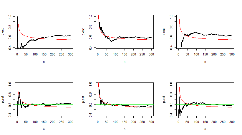
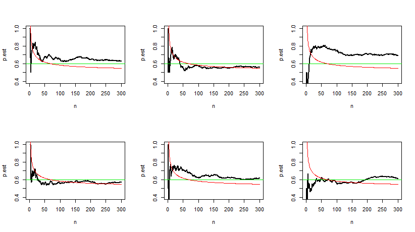
Now let's look at traces of twelve experiments at each step $1, 2, \dots, 300.$ The jagged black curves show the estimated Success probability $\hat p = X_i/i,$ for $i = 1, 2, \dots, 300.$ The red curves show critical values of the approximate normal test at each step, which are computed according to $H_0.$ Asymptotically, they approach $0.5.$

It is clear that by the time we have 300 observations (at the right of each panel) the jagged black curve (trending towards $0.6)$ is very likely to have risen above the (red) critical value.

However, in several of the twelve panels the first crossing of the black trace above the critical value occurs substantially before 300 observations have been collected. (A few of them when $\hat p$ is far from $0.6.)$ If we were to stop at the first crossing, we would not have an honest conclusion.

Sequential analysis allows for early stopping, but for legitimate early stopping the red curves have to be different (harder to cross).

Note: Here is R code for the figures. The last six runs were made using the seed shown.

set.seed(2021)
par(mfrow=c(2,3))
 for(i in 1:6){
  N=300; n = 1:N
  x = rbinom(N, 1, .6)
  p.est = cumsum(x)/n
  plot(n, p.est, ylim=c(.4,1), lwd=2,type="l")
   abline(h=.6, col="green2")
   upr = 1/2 + (1.645/2)/sqrt(n)
   lines(n, upr, col="red")
  }
par(mfrow=c(1,1))