Calculating mean follow up from ONLY sample size and range

Question

I have several observational studies (mostly historical, prior to 1950s) that are looking at relapse rate across several years of follow up period for depression. I only have MINIMUM and MAXIMUM follow up period and sample size (ie one study reports a follow up period of 10-15 years for a sample size of 208 people). However no mean follow up period is provided. I know from knowledge of the subject/relapse rate trends in modern studies on the same subject that it is a left skewed distribution- ie there will be more relapses in the early period of the study for each individual and then they will become less frequent with time.

So on this basis, ie knowing sample size, range, and type of distribution, is it possible to calculate mean follow up period? Also on STATA, since that is the software i am required to use for this project. Any help on this would be really appreciated.

Answer 1

You would need to have some idea how relapse times are distributed within the interval.

For example, if they are exponentially distributed, then the mean of a moderate number of relapse times is roughly 17% of the way from the minimum to the maximum.

Here is a simulation for 200 subjects; results for 100 and were about 19% and results for 500 were about the 15%.

set.seed(2021)
m = 10^5;  v = a = w = numeric(m)
for (i in 1:m) {
 x = rexp(200)
 v[i] = min(x); a[i] = mean(x); w[i] = max(x)
 }
mean(v); mean(a); mean(w)
[1] 0.00499292
[1] 0.9999175
[1] 5.875548
(mean(a)-mean(v))/(mean(w)-mean(v))
[1] 0.1694771

Note: For a uniform relapse distribution, results were about 50%.

Answer 2

To expand a bit on BruceET's answer, you must have some idea as to how the relapses are distributed. The exponential is a one-parameter distribution: once you know its mean, you know its variance and how all the quantiles are distributed. Anything more complex, such as a gamma or a Weibull—which are also right-tailed, left-moded distributions—will harder to solve, but if you restrict yourself to a two-parameter distribution, you may be able get an estimate.

Clearly, you have to set an assumed percentile as your seen maximum. You cannot have the entire distribution as most of these are defined for the entire real non-negative number line. While the minimum may well be the 0th percentile, that will not help us. Since 0 is the minimum for every such distribution. But if we can say it is the 1st or second, we now have two "pieces" of information: the min and the max serving as our estimates of the 2% and 98%, so we can reverse engineer the quantile functions for a given distribution to get two parameters, and thus the mean.

For example. Let's use the Pareto parameterized with shape $\alpha$ and scale. $\theta$. The CDF of the Pareto is:

$$ F(x) = p = 1 - \left(\frac{\theta}{x+\theta}\right)^\alpha $$

Which means:

$$ x = \frac{\theta}{\left(1-p\right)^\frac{1}{\alpha}} - \theta $$

If you have fixed your minimum as $p_1 = 0.02$ and your maximum as $p_2 = 0.98$ you can solve for $\alpha$ and $\theta$ and then use those parameters to estimate the mean.

Some distributions don't have closed forms without the use of special functions (gamma, beta, etc.) and so a brute force technique can be used. Forgive my use of R; I don't know stata. The following function returns the sum of the squared error between the min and the quantile representing $p_1$ and the max and the quantile representing $p_2$.

RangeErrGam <- function(par, min, max, p1, p2) {
  shp <- par[[1]]
  scl <- par[[2]]
  (min - qgamma(p1, shp, scale = scl)) ^ 2 +
    (max - qgamma(p2, shp, scale = scl)) ^ 2
}

Minimizing this error will result in parameters which can be used for estimating the mean. Let's say your minimum was 5 weeks and your maximum was 35 weeks.

fit <- optim(c(3, 10), RangeErrGam, min = 5, max = 35, p1 = 0.02, p2 = 0.98,
             method = 'Nelder-Mead', control = list(maxit = 1e4))

This results in:

> fit
$par
[1] 4.947039 3.332601

$value
[1] 6.43681e-06

$counts
function gradient 
     147       NA 

$convergence
[1] 0

$message
NULL

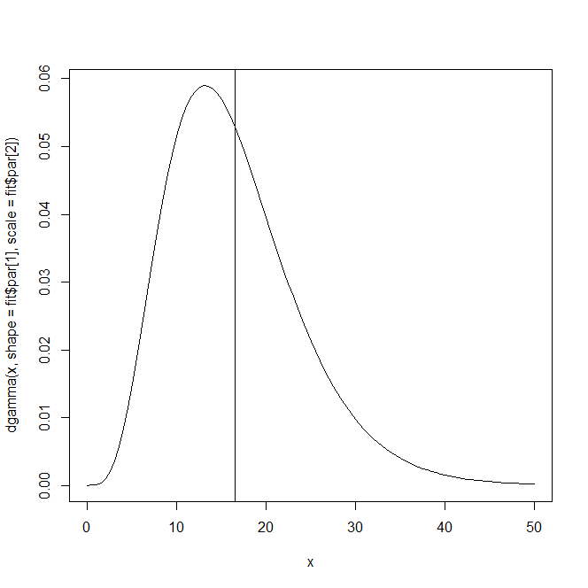
So the mean relapse time would be shape * scale or about 16.5 weeks.

Plotting this distribution shows the characteristics you wanted (left-mode, right-tail):

curve(dgamma(x, shape = fit$par[1], scale = fit$par[2]), from = 0, to = 50)
abline(v = fit$par[1] * fit$par[2])

This method can be extended to any two-parameter distribution.