Figure 3c of the paper appears to have relevant data. I have not read the paper in enough detail to know whether these are the only relevant data, so my intention here is only to reveal the nature of a meaningful answer.
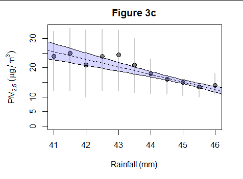
This is my version of the figure.

The caption reads, in part,
(c) ... Annual observations of dust concentrations over the Bod´el´e were divided into equal sized bins and the average annual PM2.5 concentrations (points) and interquartile ranges (gray lines) over all survey locations were calculated within each of these bins.
The points and gray lines thereby constitute a summary of the data, while the dotted line and the blue region through which it goes are part of my analysis. A dotted line also appears in the original figure and is very close to this one.
I reasoned thus: the interquartile ranges (IQRs) vary substantially across the dataset. This suggests we might be less certain about the averages with large IQRs than about averages with small IQRs. I therefore took the IQR to be a proxy for the standard errors of the averages. The fitted line is the inverse-variance weighted least squares fit, as would be appropriate under this assumption, and the blue polygonal area is a 95% confidence region for the fit. Because it's not an awful approximation to the data, let's continue to interpret the results.
Here is part of the summary of the least squares fit.
Coefficients:
            Estimate Std. Error t value Pr(>|t|)
(Intercept) 131.3009    13.6643   9.609 4.98e-06 ***
Rainfall     -2.5802     0.3038  -8.492 1.37e-05 ***
The last line indicates the slope of the response is estimated at $-2.58$ (in micrograms per cubic meter per millimeter of rainfall) with a standard error of $0.3038.$ Consequently, a change in rainfall of $5$ mm would be associated with a change in PM2.5 of $5 \times (-2.58) \approx -12.9$ micrograms per cubic meter with a standard error of $5\times 0.3038 \approx 1.52.$
An approximate two-sided 95% confidence interval can be constructed by putting bounds at a certain multiple $t$ of the standard error around the estimate. Usually, we would use the multiple determined by the Student $t$ distribution with $11 - 2$ degrees of freedom: $11$ for the $11$ data points minus $2$ for the two parameters (intercept, slope) needed to fit the line. This multiple is $2.262,$ giving a confidence interval of $-12.9 \mp 2.262\times 1.52 = [-16.3, -9.46].$
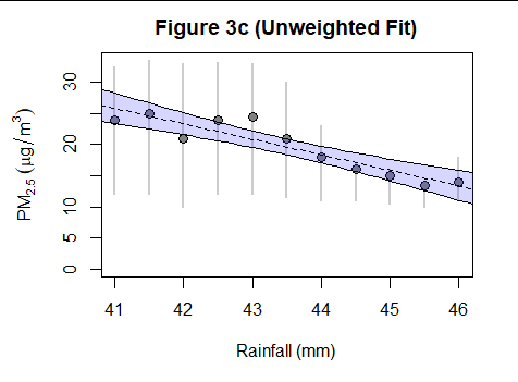
I am suspicious of these weights because an apparent rainfall histogram in the original figure suggests (without any explanation) that very little of the rainfall was observed above 44 mm. That would cause us to suspect the relative precision of the right half of the points might be far less than indicated by their narrow IQRs. To assess this, I repeated the analysis using no weights at all. Although the estimated slope barely changed (from $-2.58$ to $-2.48$), the standard error of its estimate increased to $0.36.$ The resulting confidence interval is $[-16.5, -8.36].$ That is, it is wider at the upper end, with its upper limit increasing from $-9.46$ to $-8.36.$

There aren't enough data points to support fitting a more complex model, even though the data hint that changing the rainfall in the lower area (from $41$ to $43$ mm) might be associated with no change in PM2.5 at all.
The uncertainties associated with binning the data and lack of clear descriptions of what everything in the original plot means all suggest these confidence intervals are too narrow -- but there doesn't seem to be much we can do about that.
Finally, we should be suspicious both of this analysis and of the quoted statements from the paper, because they aren't consistent. The range for the slope in the quotations ($-1.5$ to $-2$) differs from the estimates (around $-2.5$) achievable from Figure 3c and is too narrow for the standard errors of $0.3$ to $0.36$ associated with that figure. Unless you can locate a passage in the paper to explain this discrepancy, use all of its results with care and consider contacting the authors for clarification.
For the record, and for further analysis, here are the numerical values I used (given as an R expression).
X <- data.frame(Rainfall=seq(41, 46, by=0.5),
                PM2_5 = c(24, 25, 21, 24, 24.5, 21, 18, 16, 15, 13.5, 14),
                Q3 = c(32.5, 33.5, 33, 33.25, 33, 30, 23, 17, 16, 14, 18),
                Q1 = c(12, 12, 10, 12, 12, 11.5, 11, 11, 10.5, 10, 11))
The least squares output (for the weighted fit) was obtained with
summary(lm(PM2_5 ~ Rainfall, X, weights = 1/(Q3-Q1)^2))


