Kolmogorov-Smirnov Test in Python weird result and interpretation

Question

I have difficulties to understand how the Kolmogorov-Smirnov Test works. If I want to know if my samples are from a specific distribution (for example from the weibull distribution) I can compare my significance level to the p-Value I get from scipy.stats. If the p-Value is higher than my chosen alpha (5%) my samples are from the distribution. If p-Value is < 5% they are different.

In this code example I don't understand the result. My sample are from the same distribution i test against and I get a p-Value of 0 which means they are from a different distribution which makes no sense to me. It would be great if someone could help me out with this.

import scipy.stats as stats
import numpy as np

smapleData = stats.weibull_min.rvs(2.34, loc=0, scale=1, size=10000)
x = np.linspace(0, max(tmp), num=10000, endpoint=True)

stats.kstest(stats.weibull_min.pdf(x, 2.34, loc=0, scale=1), smapleData)

#-> KstestResult(statistic=0.5031, pvalue=0.0)

I read that the KS-test might not be great for large Data. If someone would have an other idea how I can compare to Sample sets (without knowing the distribution behind it) how similar they are I would appreciate it.

Answer 1

You got a couple of things wrong while reading the documentation of the Kolmogorov-Smirnov test.

First you need to use the cumulative distribution function (CDF), not the probability density function (PDF). Second you have to pass the CDF as a callable function, not evaluate it at an equally spaced grid of points. [This doesn't work because the kstest function assumes you are passing along a second sample for a two-sample KS test.]

from functools import partial

import numpy as np
import scipy.stats as stats


# Weibull distribution parameters
c, loc, scale = 2.34, 0, 1
# sample size
n = 10_000

x = stats.weibull_min.rvs(c, loc=loc, scale=scale, size=n)

# One-sample KS test compares x to a CDF (given as a callable function)
stats.kstest(
    x,
    partial(stats.weibull_min.cdf, c=c, loc=loc, scale=scale)
)
#> KstestResult(statistic=0.0054, pvalue=0.9352)

# Two-sample KS test compares x to another sample (here from the same distribution)
stats.kstest(
    x,
    stats.weibull_min.rvs(c, loc=loc, scale=scale, size=n)
)
#> KstestResult(statistic=0.0094, pvalue=0.9291) 

---

@Dave is correct that with hypothesis testing we don't accept the null hypothesis, we can only reject it or not reject it. The point is that "not reject" is not the same as "accept".

On the other hand, it sounds a bit awkward to say "we have a sample of 10,000 but we simply have insufficient evidence to conclude anything". At this sample size we expect that estimates are precise (have small variance).

Note that this situation is a bit hypothetical. In practice we rarely know the true distribution or that two large samples come from the same distribution as in the simulation. So in the real world, at sample sizes on the order of 10k, it's more likely that the p-value is small, not large.

So do we learn anything if the sample size is large and the p-value is large?

• We learn that the significance level α = 0.05 doesn't make sense for large data. Keeping α fixed while n grows implies we are looking for smaller and smaller effects.
• And we learn that — while we cannot accept the null hypothesis as true — the evidence is consistent both with "no effect" and with "trivial effect". If we have chosen the sample size so that we have enough power to detect differences of interest to us, then we also have a good idea what "trivial" means.

You can read more on the topic Are large data sets inappropriate for hypothesis testing?.

Answer 2

In addition to the coding mistakes addressed in the other answer, there are two statistics mistakes in the post that I want to address.

If the p-Value is higher than my chosen alpha (5%) my samples are from the distribution.

This is a common misinterpretation of the p-value. We do not accept null hypotheses. When the p-value is larger than $\alpha$, we simply have insufficient evidence to conclude anything. Otherwise, you could just collect two points, conduct your test, pretty much never reject, and keep claiming that you're proving null hypothesis after null hypothesis. Further, this logic applies to all hypothesis testing, not just KS.

I read that the KS-test might not be great for large Data.

There is some truth to this that is discussed extensively in another Cross Validated post. While that question addresses the normal distribution, the logic applies. Summarizing the link, large sample sizes give hypothesis tests (not just KS) great power to detect small differences that are not of practical importance or of interest to clients/customers/reviewers/bosses. However, that only happens when the null hypothesis is slightly incorrect, say a null hypothesis of $\mu = 0$ when the real $\mu = 0.1$. If the null hypothesis is true, the KS test does exactly what it is supposed to, as I will demonstrate in a simulation.

library(ggplot2)
set.seed(2022)
B <- 5000
N <- 25000
ps <- rep(NA, B)
for (i in 1:B){
  
  # Simulate some Weibull data
  # 
  x <- rweibull(N, 2.34, 1)
  
  # KS-test the data for having the specified Weibull distribution
  #
  ps[i] <- ks.test(x, pweibull, shape = 2.34, scale = 1)$p.value
  
  if (i %% 25 == 0 | i < 5 | B - i < 5){
    print(paste(i/B*100, "% complete", sep = ""))
  }
}
d <- data.frame(ps = ps, CDF = ecdf(ps)(ps), Distribution = "Weibull")
ggplot(d, aes(x = ps, y = CDF, col = Distribution)) +
  geom_line() +
  geom_abline(slope = 1, intercept = 0) +
  theme_bw()

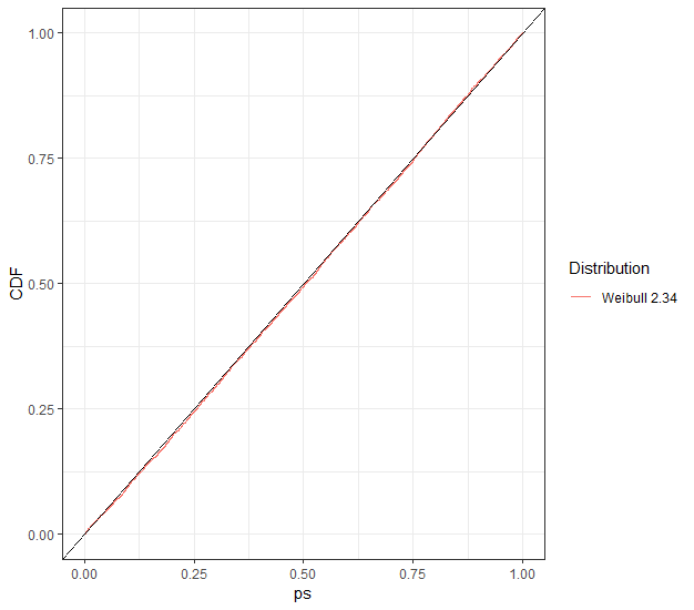
Since the null hypothesis is true, the KS test rejects approximately the correct number of times (for any $\alpha$-level, not just $0.05$), as the $U(0,1)$-looking CDF of the p-values shows. I even supercharged the KS test by having a sample size of $25000$, as opposed to your $10000$, yet KS was not overpowered.

Now let's tweak the simulation ever so slightly. A plot above the $y=x$ diagonal line indicates power to detect the difference.

library(ggplot2)
set.seed(2022)
B <- 5000
N <- 25000
ps <- rep(NA, B)
for (i in 1:B){
  
  # Simulate some Weibull data
  # 
  x <- rweibull(N, 2.34, 1)
  
  # KS-test the data for having the specified Weibull distribution
  #
  ps[i] <- ks.test(x, pweibull, shape = 2.3, scale = 1)$p.value
  
  if (i %% 25 == 0 | i < 5 | B - i < 5){
    print(paste(i/B*100, "% complete", sep = ""))
  }
}
d <- data.frame(ps = ps, CDF = ecdf(ps)(ps), Distribution = "Weibull 2.3")
ggplot(d, aes(x = ps, y = CDF, col = Distribution)) +
  geom_line() +
  geom_abline(slope = 1, intercept = 0) +
  theme_bw()

I won't tell you if you should care about $2.3$ vs $2.34$, but even if you don't, the KS test sure does!