1
$\begingroup$

I would like to analysze the relation between my continuous response 'soil moisture content [%]' and 2 categorical and 1 continuous predictors. I fit a linear mixed model and checked the distribution with the check_distribution() function of the performance package.

library(performance)

lmer(soil_moisture ~ weed_coverage+distance  + 
    treatment + (1 | kettlehole/plot) + 
    (1|date), data = BFK_comp) -> lmmod

check_distribution(lmmod)

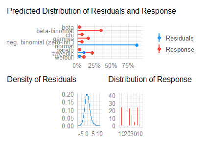
I got this result and plot

Predicted Distribution of Residuals

 Distribution Probability
       normal         88%
      tweedie          9%
      weibull          3%

Predicted Distribution of Response

  Distribution Probability
 beta-binomial         34%
       tweedie         22%
         gamma         16%

enter image description here

As I understand it, the predicted distribution of the residuals need to be normally distributed, so I can use a linear regression, right? I am not talking about the other assumptions here, just normality. After that I did a test with the check_normality() fuction, also from the performance package and it says

Warning: Non-normality of residuals detected 
           (p < .001).

These results seem to be contradictory to me or am I missing something here?

Also, I want to test if there is a significant difference between soil moisture content and distance (factor with 2 levels). Do I need to look at the distribution of the response or at the distribution of the residuals to find out if I need to use a t-test or wilcoxon signed rank test?

$\endgroup$
11
  • $\begingroup$ Your response is only defined in the inverval [0, 1]. Therefore, the residuals cannot be normal distributed. However, the normal distribution can still be a sufficient approximation. I would consider using beta-regression. The only issue is that this does not allow observed values of exactly 0 or 1. But then, you could argue that soil moisture cannot be exactly 0 or 1. $\endgroup$
    – Roland
    Commented Apr 29, 2022 at 10:34
  • 1
    $\begingroup$ I suspect what is going on is that you have a sample size that's large enough that the hypothesis test is returning a significant result ---- there is good evidence that the residuals deviate from a normal distribution ---- even though the residuals may be reasonably approximately normal. This is one reason why using a hypothesis test to assess model assumptions isn't the best approach. You are better off looking a plot of the residuals, as a histogram, density, or q-q plot. $\endgroup$ Commented Apr 29, 2022 at 18:25
  • $\begingroup$ With the two-sample problem you raise at the end of the question: For me, I'd just as soon use a regression model with a single categorical variable on the right hand side, and then look at the residuals. But you could also look at the distribution and spread of the two groups. P.S. You might have meant the Wilcoxon rank sum test. $\endgroup$ Commented Apr 29, 2022 at 18:29
  • $\begingroup$ Oh, I might have misunderstood that question about comparing between levels of distance. If that variable is part of the larger model, assess the larger model for appropriateness. And then use the emmeans package to compare among the terms you are interested in. Model types supported by emmeans are listed here: cran.r-project.org/web/packages/emmeans/vignettes/models.html $\endgroup$ Commented Apr 29, 2022 at 18:34
  • $\begingroup$ Thanks for your answers. I still dont understand in which cases I need to look at the predicted distribution of the residuals and in which cases at the predicted distribution of the response. $\endgroup$
    – Effigy
    Commented Apr 30, 2022 at 9:43

1 Answer 1

1
$\begingroup$

Answer mostly from comments:

  • (Roland) Your response is only defined in the interval [0, 1]. Therefore, the residuals cannot be normal distributed. However, the normal distribution can still be a sufficient approximation.

  • (Roland) I would consider using beta-regression. The only issue is that this does not allow observed values of exactly 0 or 1. But then, you could argue that soil moisture cannot be exactly 0 or 1.

  • (WHuber) Ultimately, the answer to your question is afforded by the model you are using. Almost any regression model makes assumptions about the conditional response distribution, but not about the marginal response distribution.

  • (Sal) I suspect what is going on is that you have a sample size that's large enough that the hypothesis test is returning a significant result ---- there is good evidence that the residuals deviate from a normal distribution ---- even though the residuals may be reasonably approximately normal.

  • (Sal) This is one reason why using a hypothesis test to assess model assumptions isn't the best approach. You are better off looking a plot of the residuals, as a histogram, density, or q-q plot.

  • (Sal) If you want to compare among levels of a variable that is part of the larger model, assess the larger model for appropriateness. And then use the emmeans package to compare among the terms you are interested in. Model types supported by emmeans are listed here: cran.r-project.org/web/packages/emmeans/vignettes/models.html

  • (Sal) If your model is a type of general linear model (lm), you'll see that the model specifies that the errors are normally distributed. One method to assess this is to look at the residuals. As I mentioned, don't use hypothesis tests to look at this assumption. Other tests like anova, ancova, t-test, linear regression can be thought of as an lm. It makes life simple to think of these tests this way, and not worry if the data should be normally distributed.

To give an example of this final comment, we can look at two independent groups to assess the distribution of values and equal variance before a t-test.

set.seed(sum(utf8ToInt("Salvatore")))
 
A = rnorm(50, 10, 1)
B = rnorm(50, 12, 1)
Y = c(A, B)
Group = c(rep("A", length(A)), rep("B", length(B)))
Data = data.frame(Group, Y)
 
library(lattice)
 
histogram(~ Y | Group, data   = Data,
           layout = c(1,2))

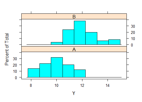
Histograms of each group

From these histograms, the distribution in each group is relatively bell-shaped, but with some skew. The spread of the data is each group is relatively similar.

As an alternative, we could formulate the t-test as a general linear model, and then assess the residuals.

 model =lm(Y ~ Group, data=Data)
 
 hist(residuals(model))
 
 plot(predict(model), residuals(model))

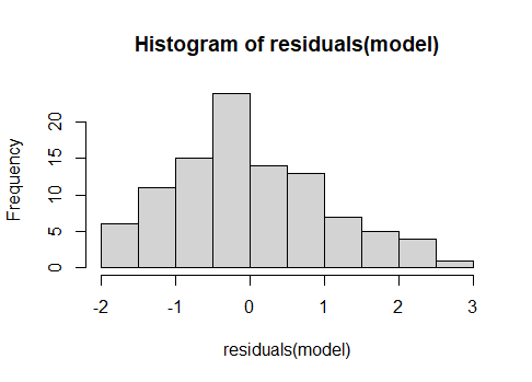
Histogram of model residuals

Here, the residuals are somewhat right-skewed.

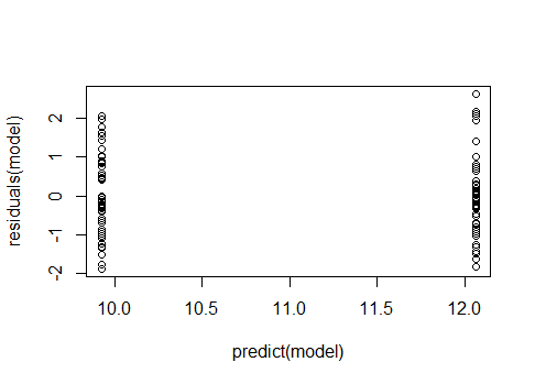
Plot of residuals versus predicted values

The residuals are fairly homoscedastic when plotted against predicted values.

$\endgroup$

Your Answer

By clicking “Post Your Answer”, you agree to our terms of service and acknowledge you have read our privacy policy.

Not the answer you're looking for? Browse other questions tagged or ask your own question.