So you have two populations, $a$ and $b$. In each, you want to estimate the proportion $P$ of made payments. (Then $1-P$ is the proportion of missed payments.)
Simple method
The easiest way to do this is to count all made payments in each population, and divide by total number of desired payments in each population. In math terms, you have for population $a$
$$p_a = m_a/M_a$$
where $m_a$ is the number of made payments in population $a$, and $M_a$ is the number of opportunities for payments in population $a$. The same thing goes for $b$.
In order to test whether $p_b$ is significantly larger than $p_a$, you have to know the variance of these estimations. The neat thing about this direct method is that the variance of $p_A$ is just
$$s_{p_a}^2 = \frac{p_a(1-p_a)}{M_a-1}$$
Obviously, it's the same thing for $b$. The variance of $p_b - p_a$ is the sum of the variances of each, and this can be compared to the difference.
Example
Say that in conclusion, population $a$ made 213 payments out of 253, and population $b$ made 43 payments out of 49. Then you have
$$p_a = \frac{213}{253} = 0.84$$
and
$$p_b = \frac{43}{49} = 0.88$$
This looks like an improvement! The treatment group made their payments 4 percentage points more often!
You also get the variances
$$s_{p_a}^2 = \frac{0.84 \cdot 0.16}{252} = 0.0005$$
and
$$s_{p_a}^2 = \frac{0.88 \cdot 0.12}{49} = 0.002$$
The difference between the proportions (the effect size you see) is
$$d = p_b - p_a = 0.04$$
and the variance of this is
$$s_d^2 = s_{p_a}^2 + s_{p_b}^2 = 0.0025$$
The standard error is the square root of the variance:
$$\textrm{se}_d = \sqrt{0.0025} = 0.05$$
In other words, the effect we observed, improvement of 0.04, is less than one standard error. Definitely not a significant result.
Sample size
You can probably simplify the sample size calculation, by assuming that you know $p_a$ to fairly high accuracy and it won't contribute significantly to the variance of the estimated effect size. (If that's wrong, you'll have to include the extra term to account for the variance of $p_a$.)
We can go backwards from the previous result to find the required sample size. It depends on three things:
The baseline $p_a$ for the control group. You probably have a fairly good idea about what this number is, but I don't, so I'll assume $p_a = 0.84$.
How large an effect you want to show. Again, I don't know how much this voucher campaign costs, so I have no idea. But let's say you need to show an effect size at least $d = 0.1$ for it to be worth it.
At what confidence level you want it. Also not my place to decide, but to get anywhere, let's say you want a confidence level of $0.05$. Under a somewhat reasonable normality assumption, this translates to an effect larger than 1.645 standard errors.
Combining some equations from above
$$\frac{(p_a + d)(1-(p_a + d))}{x - 1} = \left(\frac{d}{1.645}\right)^2$$
where $p_a$ is the baseline proportion from the control group, $d$ is the desired effect size, and $x$ is the sample size for the treatment group.
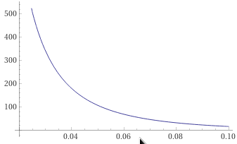
If we solve this equation for the above numbers, we get a required sample size of 17. This might sound smaller than you expected, but that is because we are trying to show such a large effect. If an effect of magnitude 0.1 is indeed there, it will be apparent from even just a small sample.
If you're happy with an effect of just 0.05, you need just over 100 samples. It drops fairly rapidly the larger an effect you want to show:

Duration
The duration should be long enough that you manage to collect the required sample size to show the effect you want to show. How long that is depends on how many customers you have, and how often they have to pay you. The moment the last person has either made their payment or definitely missed it, you can stop the experiment.
If you need to estimate the duration ahead of time, that is starting to become a separate problem estimation problem from the one you are primarily asking in this question, and perhaps warrants its own question.
Mean of means
Now that you know the simple method, I want to say that what I've described above only works when you have $m_b$ and $M_b$. You were suggesting collecting only the proportions $p_{b,i} = m_{b,i}/M_{b,i}$.
The drawback of this is that the result will be much harder to interpret. In the previous simple case, we could say that if $p_b = p_a + 0.08$ then we had observed an 8 percentage point improvement in the treatment group. We can't say that with the data you suggested, because if one person is a really frequent customer (100s of payments) and goes from paying almost none of them on time to all of them on time, that, in a sample of 50, still only counts for 1/50 of the mean.
In other words, you will no longer be able to talk about the effect size in a way that means anything to a business person.
If you still want to do it, go ahead. The variance of each individual $p_{b,i}$ is computed the same way as in the simple case. Then when you take the mean of the $p_{b,i}$, the variance of that mean will be the sum of the variances divided by the number of $p_{b,i}$.
Other measurements
You could argue that the design I've proposed also suffers from the same "premature aggregation" problem that the mean-of-means design does.
There could be regulatory reasons that the proportion of made payments matters. But what probably matters to the business is the amount of money past due. Think about it: both Steve and Sue could have the exact same proportion of missed payments, say, 1 of 10, but maybe Steve has a missed payment of \$1543 and Sue's is only \$19. The former probably hurts the business more.
So there's a third design for you, if it's possible: measure the amount of money past due instead.

