What qualifies as "slight violation" of proportional hazards?

Question

I'm using Cox survival analysis to find predictors of mortality in a health dataset.

Although Cox assumes proportional hazards of the variables, my reading tells me that "slight violations" of this assumption are not a big deal.

1. I would like to know what qualifies as "slight" in this case.

2. It seems that log-log plots can help in the case of categorical variables; is there an equivalent for continuous?

3. Can this also be deduced from Schoenfeld plots alone? For example, I see that Chen writes that, although heart rate is statistically significant when testing the PH assumption, visual inspection of the Schoenfeld plot suggests that the violation is small. In my case, many of the Schoenfeld plots of my significant variables have much straighter lines than that (although my dataset is large, >100 000). Below I put one of my own as a reference, and this is rather representative of plots for the other variables too.

4. If possible from the information provided, could we conclude that this violation is also small and therefore proceed with analysis as normal, without adding interaction terms or changing the test?

Answer 1

Only you and your colleagues can answer the question in the title, based on your understanding of the subject matter. Here's how I would start to approach it.

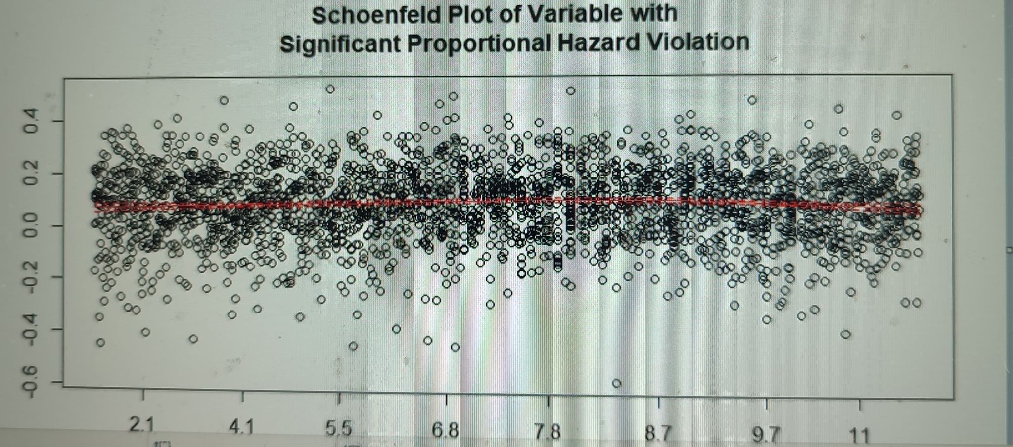
In your plot, it looks like the coefficient estimate is slightly below 0.1 at early times, and drops off a bit at later times. It would help to add a horizontal line at the overall coefficient estimate from the model.* Let's say the estimate at early times is $\beta(\text{early}) = 0.08$, that at late times is $\beta(\text{late}) = 0.05$, and the coefficient returned by the model overall is $\beta=0.065$.

That corresponds to a hazard ratio of 1.067 for the model's overall estimate, versus 1.083 for early times and 1.051 for late times. How practically significant are those differences?

I think that addresses specific questions 1,3, and 4.

With respect to continuous predictors, I'd first worry about modeling them with adequate flexibility. It's unrealistic to expect an exact linear association of such a predictor with the log-hazard of an event. Mis-specifying the association with outcome can show up as an apparent violation of proportional hazards (PH). See this page for an example. With this size data set you can have a lot of flexibility in modeling individual predictors and potential interactions.

Table 20.9 of Frank Harrell's Regression Modeling Strategies summarize strengths and weaknesses of several approaches to evaluating PH. For a continuous predictor you could use categorical log-log plots for PH on cases grouped by quantiles of their values.

Alternatively, you could include properly modeled interactions of the covariate with time in the model, as described near the end of Section 20.6.2 of that book, and evaluate the significance of the interactions with time. That's equivalent to the modeling of time-varying covariates explained in Section 4.2 of the R survival package time-dependence vignette. It might be computationally expensive for your large data set.

But even after you've done all that, the fundamental question is still one that only you and your colleagues can answer: is the violation of PH large enough to matter for your application?

---

*Although this is called a "Schoenfeld residual plot," the plot is of the time-dependent estimates of the regression coefficient, residuals added to the overall model coefficient. The coefficient returned by the full model can be considered a type of average.