log transform fixed PH in Cox model - how?

Question

I have survival data to which I am fitting a Cox model with a continuous predictor. The cumulative martingale residual method (supremum test) of Lin, Wei and Ying suggested that both proportional hazards (PH) and functional form assumptions of the predictor were significantly in error. I log transformed the predictor and the functional form p-value improved (now non significant) but the p-value for the PH assumption is now also non-significant indicating no significant deviation from PH. How can this be ? How can transforming a predictor make the hazard ratio between different levels of the predictor constant over time ??

Answer 1

If you don't specify the correct linear form for a continuous predictor in a Cox proportional hazards (PH) model, it's quite possible to get this behavior. Tests for PH come after the regression coefficients for the predictors have been estimated. If there is an error in the model for the regression coefficients then that error can also lead to failure of a PH test.

Consider the Schoenfeld residuals, each of which is the difference between the observed predictor value and the predictor value expected from the Cox model, based on the observed event time. If you don't specify a correct linear form for the continuous predictor, then the Cox regression will be approximating a true non-linear relation with a linear relation. That will necessarily lead to residuals between observed and expected predictor values. If there is a trend in those residuals over time, then that trend will provide evidence against the PH assumption. Using the correct transformation to meet the linearity requirement can prevent both problems.

A simple example illustrates this with analysis based on linear regressions. Let's say that you know that the hazard for each individual is constant in time; that is, survival times fit exponential distributions. A predictor $z$ (which might represent a transformation of the originally measured predictor values $x$) has the standard linear relation assumed by a Cox model, so that that the fraction surviving over time is:

$$S(t) = \exp(-\lambda \exp(\beta z)t)$$ or $$\log S(t)= -\lambda \exp(\beta z) t$$

Say you have known values of $z$ and enough individuals examined for each value that you have precise estimates of the corresponding median survival times. Call those median survival times $T_{50}$ values. Then the $T_{50}$ values bear a simple relation to $z$, as $S(T_{50})=1/2$:

$$\log(T_{50})= \log (-\log (1/2))- \log \lambda-\beta z $$

So if $z$ meets the linearity assumption, a plot of $\log (T_{50})$ against $z$ will give a straight line with a slope equal to the negative of $\beta$, the regression coefficient for $z$, and with the intercept providing information about the baseline hazard value $\lambda$ when $z=0$.

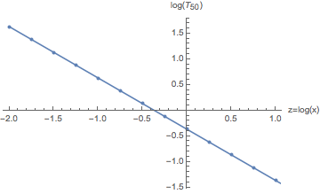
Now let's apply this to the situation in the OP. We have measured predictor variable values $x$, but they need to be transformed to $z=\log x$ to meet the linearity requirement for the Cox regression. If we do the plot suggested above on this log-transformed scale (with $\lambda =1$ and $\beta = 1$ as an example), we get a straight line with slope of -1:

Note that the observed and predicted values of the predictor on this scale agree. If instead we omit the log transform of $x$ and try the same plot we get:

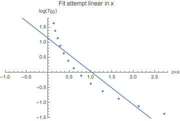
where the points are the actual values and the solid line represents an attempt at a linear least-square fit. This isn't how the Cox PH model fitting works but the basic idea is the same: you try to find the best linear approximation to this inherently non-linear relation with the predictor values.

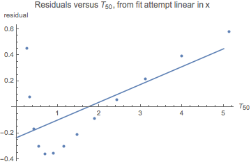
Note that the horizontal distance between each point and the solid line is the residual between the observed value of $x$ and the value expected based on this attempt at a linear fit. Now plot the values of those residuals against the untransformed $T_{50}$ values, which is one way to evaluate the PH assumption:

The straight line shows the linear least-squares trend of this decidedly non-linear relationship between residuals and median survival times. This plot would argue that the PH assumption doesn't hold as there is a clear trend in residuals over time. Again, this analysis based on median survival times isn't how standard tests for PH are done for Cox models. Nevertheless the implication is clear: if you don't specify the correct form of a relationship between a continuous predictor and outcome, the failure to meet the linearity assumption can also lead to failure to pass a PH test.

Answer 2

This paper (Proportionally Difficult: Testing for Nonproportional Hazards in Cox Models) covers this topic nicely

From page 190

The power of the test to detect nonproportionality is dependent on the correct specification of the model. Specifically, omitted covariates and interactions as well as nonlinear functional forms can appear as violations of the proportional hazards assumption complicating the detection of nonproportionality.

And from page 204

The standard test, the Therneau and Grambsch nonproportional hazards test, sees widespread use as it is easy to conduct and interpret. Unfortunately, application of the standard test requires some care as it is sensitive to several forms of misspecification. Analysts must be aware that omitted predictors, omitted interactions, and nonlinear covariate functional forms can all trigger a significant result from the test. Correcting nonlinear functional forms is an important way to improve the specification before testing for nonproportional hazards.