Its probably best we do this with a concrete example. I'll generate a little problem in Stan and we can answer some of these together. Here is some code to set up the problem. We'll draw some observations from the following process
$$ y_i = 2x_i + 1 + \epsilon_i $$
$$ \epsilon_i \sim \mbox{Normal}(0, 0.3^2) $$
The model we will use is
$$ \mu = \beta_1 x + \beta_0 $$
$$ y_i \sim \mbox{Normal}(\mu, \sigma) $$
Here, I have not placed priors on $\beta_1, \beta_0, \sigma$ yet. I'm going to let the software do that for me and sweep the problem under the rug.
library(tidyverse)
library(rstanarm)
library(tidybayes)

x <- rnorm(10)
y <- 2*x + 1 + rnorm(10, 0, 0.3)
d <- tibble(x, y)
We can fit the model with
fit <- stan_glm(y~x, data=d, family = gaussian())
The result of the model is not a point estimate. They are samples from the posterior. We can extract those samples with
fit %>%
  spread_draws(`(Intercept)`, x, sigma) %>%
  rename(b0=`(Intercept)`, b1=x)

# A tibble: 4,000 × 6
   .chain .iteration .draw    b0    b1 sigma
    <int>      <int> <int> <dbl> <dbl> <dbl>
 1      1          1     1 0.919  1.97 0.352
 2      1          2     2 0.924  1.98 0.352
 3      1          3     3 0.922  1.99 0.337
 4      1          4     4 0.969  1.95 0.310
 5      1          5     5 0.941  2.02 0.331
 6      1          6     6 0.969  1.93 0.321
 7      1          7     7 0.968  1.94 0.324
 8      1          8     8 0.935  2.00 0.345
 9      1          9     9 0.937  1.97 0.342
10      1         10    10 0.943  2.00 0.299
# … with 3,990 more rows
Each row in this dataframe is a draw from the joint posterior distribution.
Are we not trying to maximise the log probability at each iteration to converge towards the best possible values for these 2 parameters?
No. Right now, all we have done is obtained samples from the model. The loglikelihood does play a role in the computation of the posterior, but we are not maximizing anything. We are simply drawing from the posterior, and remember -- the result from a Bayesian model is not a point estimate, its a distribution.
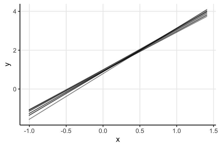
Distributions are hard to reason about. Let's put these draws in context by visualizing some of the estimates. For the first couple of draws in the dataframe, above, I'm going to draw a line.

Now, that isn't very useful. People often want one number to summarize things. We could take the pointwise mean of each of these lines and use that as our prediction.
...why is this not optimization?
It is optimization in a sense that the sample mean minimizes the squared error of the estimate. Or we could have used the median which optimizes a different loss. Or some other estimate which would minimize some other function.
The important part here is that the optimization does not occur in the model fitting stage. It occurs post facto, once we have the model.
If not, what are we doing exactly and how are we obtaining these "best-fit" values?
It depends on how you define 'best'. 'Best' under what conditions? If we want the best estimate (where best is minimal squared error) then we use the sample mean.
In this example, is the Markov Chain simply the prior distributions from which we sample our 2 parameters?
Posterior distribution, not prior. The chain represents samples from this distribution.

