Is asymptotic unbiasedness different from unbiasedness in practice?

Question

Given some estimator T for a parameter θ, by definition T is unbiased if its bias B(T) is 0. It is asymptotically unbiased if B(T) is not 0, but some value that tends to 0 as n goes to infinity. My question is: how are these properties different in practical terms? Unbiasedness by itself is only true for infinitely large n: given that B(T) = E(T) - θ, and the expected value E(T) is the mean of T's values over infinitely large n, it would seem that the two properties are saying the same thing. So, given they have the same variance, how do you distinguish between an estimator:

1. whose sampling average tends towards θ for large n [E(T) = θ, unbiased]
2. whose sampling average tends towards some value that tends towards θ for large n [E(T) = θ + f(n), where f(n) tends to 0 for large n, asymptotically unbiased]

Answer 1

Let $X_1,\dots,X_n\overset{iid}{\sim}N(\mu, 1)$, so the sample size is $n$.

Define two estimators of $\mu$.

1. $\hat\mu_1 = \bar X = \dfrac{1}{n}\sum_{i=1}^n X_i$

2. $\hat\mu_2 = \bar X = \dfrac{1}{n} + \dfrac{1}{n}\sum_{i=1}^n X_i$

Let's calculate the expected value of each.

$$ \mathbb E\left[\hat\mu_1\right] = \mathbb E\left[\dfrac{1}{n}\sum_{i=1}^n X_i\right] \\=\dfrac{1}{n}\mathbb E\left[\sum_{i=1}^n X_i\right] \\=\dfrac{1}{n}\mathbb \sum_{i=1}^nE\left[ X_i\right] \\=\dfrac{1}{n}\mathbb \sum_{i=1}^n\mu \\=\dfrac{1}{n} n\mu \\=\mu $$

For any finite number of samples, including just one sample, $\bar X$, the usual sample mean, is unbiased.

$$ \mathbb E\left[\hat\mu_2\right] = \mathbb E\left[\dfrac{1}{n}+\dfrac{1}{n}\sum_{i=1}^n X_i\right] \\=\dfrac{1}{n} + \dfrac{1}{n}\mathbb E\left[\sum_{i=1}^n X_i\right] \\=\dfrac{1}{n} + \dfrac{1}{n}\mathbb \sum_{i=1}^nE\left[ X_i\right] \\=\dfrac{1}{n} + \dfrac{1}{n}\mathbb \sum_{i=1}^n\mu \\=\dfrac{1}{n} + \dfrac{1}{n} n\mu \\=\dfrac{1}{n} + \mu $$ There is no finite $n$ for which $\hat\mu_2$ is unbiased, since there's always some little positive number added to $\mu$. However, as $n\rightarrow\infty$, that little positive number gets smaller and smaller, vanishing in the limit. Consequently, $\hat\mu_2$ is asymptotically unbiased.

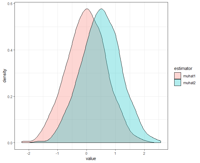
I think you are mixing up the sample size and the number of times samples are drawn. We can draw finite sample sizes over and over. For instance, I will apply the above estimators in a simulation that draws two observations $1000$ times.

KEY POINT: The sample size is two, not $1000$ or $2000$.

library(ggplot2)
set.seed(2022)
n <- 2
R <- 1000
mu <- 0

muhat1 <- muhat2 <- rep(NA, R)
for (i in 1:R){
  
  x <- rnorm(n, mu, 1)
  muhat1[i] <- mean(x)
  muhat2[i] <- mean(x) + 1/n
  
}
d1 <- data.frame(estimator = "muhat1", value = muhat1)
d2 <- data.frame(estimator = "muhat2", value = muhat2)
d <- rbind(d1, d2)
ggplot(d, aes(x = value, fill = estimator)) +
  geom_density(alpha = 0.3) +
  theme_bw()

Even with a sample size of two, the distribution of $\hat\mu_1 = \bar X$ is centered around the true $\mu=0$.

However, the sample size is two, not $1000$. We do $1000$ replications of the draw of two in order to create a distribution, not because the sample size is $1000$ or $2000$. The estimators each apply to samples with sample sizes of two.