I am struggling with assessing the best weighted regression type/model specification for my problem.
The goal is to determine influence of independent variables towards the outcome (dependent variable), so estimators and their standard errors should not be biased.
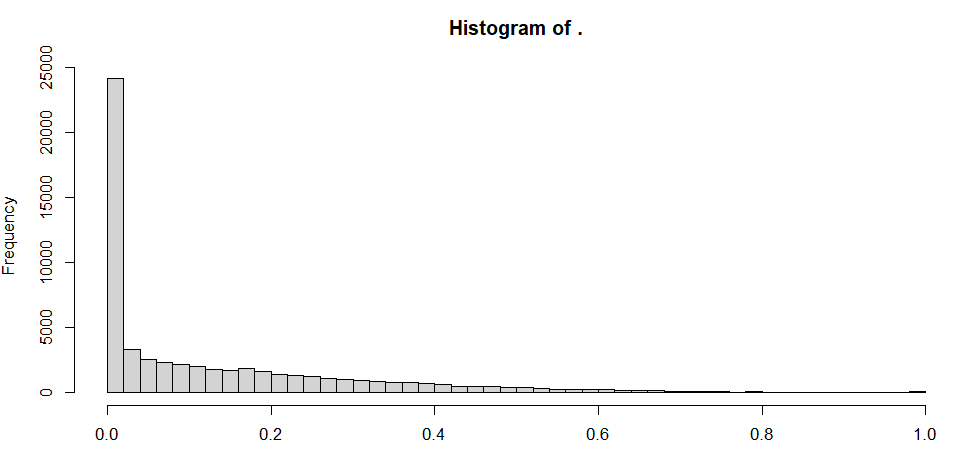
Dependent variable is a proportion (so ranging between 0 and 1), while close to zero means worse outcome of observed phenomenon. However, observations close to 1 are mostly outliers, which behaviour is comparable with lower outcomes (near zero).
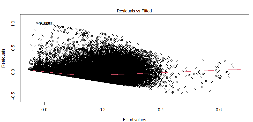
When applying weighted linear regression, some of the predicted values are outside the interval for possible outcomes (fitted values less than zero). I assume this is causing an assumption violation of autocorrelation in residuals - see graph 2 (AR tested by Breusch–Pagan test and ACF plot). Can this assumption be right?
Also searched for different types of regressions to deal with this problem. I tried to apply GLM with family distribution which corresponds with distribution of dependent variable (tried package fitdistrplus in R, but none of distributions available here are close to the outcome variable).
Independent variables have no sigmoidal relationship with the dependent variable, so I assume the GLM with binomial log link and beta regression is not suitable for this problem (Am I wrong??).
Regression needs to be weighted as it comes from significant assumptions of data.
Independent variables are:
- x1 = categorical with 7 lvls
- x2 = nominal variable with more than 30 lvls
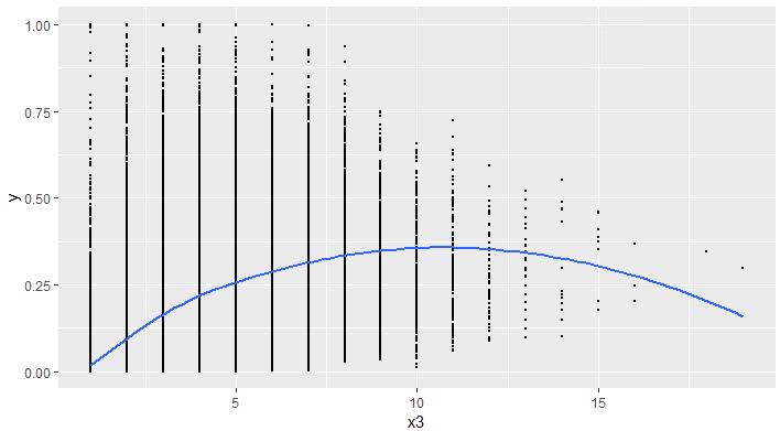
- x3 = count of occurrences (logarithmic/linear relationship with dependent variable)
- x4 = Standardized variable ranging from 0 to 1 ()
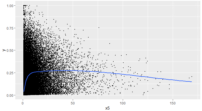
- x5 = continuous variable (growth curve with asymptote)
Can you please help me with assessing the best way to model the data? Or at least point out the way I should be looking at this problem?
EDIT:
To supplement more information regarding the data. I am trying to examine what affects the effectiveness of public procurement contracts (from specific point of view)
This is dataset after removing outliers. They were identified by isolation forest. There was need to take into account different behavioral patterns which are present in the data.
Dependent variable (proportion) = (final price of a contract minus estimated price of a contract)/estimated price of a contract. Describes how effective the procurement was, proportional amount of funds being saved.
Independent variables:
- (x1) Ordinal values with 7 lvls = Describing different mean values when observation belongs to a given category, expected result is, that with higher ordinal level raises also the dependent variable
- (x2) Nominal with more than 30 lvls = Describing different mean values when observation belongs to a given category, control variable.
- (x3) count of occurrences = How many contractors attended the contract
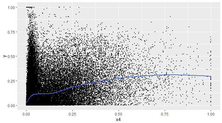
- (x4) Standardized values = Min Max Standardization of another (fully independent) proportional value on groupby lvl of x2 variable.
- (x5) continuous variable = describes mean bid count per contractor in a contract. Growth curve with asymptote is derived from the graph below. Describes competitiveness in a contract, which as I expect, has some limitation regarding the effect on a dependent variable.
Below you can see weighted loess on three input variables to see their dependence to the outcome.

