4
$\begingroup$

Problem statement:

I am using a simple linear regression with outcome $y$ and single predictor $x$ of the form:

$$ y_i \sim N(\mu_i, \sigma) \\ \mu_i = \beta_0 + \beta_1x_i $$

I assume fitting $\beta_0, \beta_1$ with maximum likelihoood (although if other method works better for the purpose of this question, I can use that). Then, I observe a new set of outcomes $\bar{y}$ for a (known) new set of predictors $\bar{x}$ which I assume come from the same process. I then assume a regression is fitted independently to $\bar{x}, \bar{y}$ obtaining $\bar{\beta}_0, \bar{\beta}_1$.

Is there an analytical way to use the original fit to get something like a "prediction interval" for $\bar\beta_1$? I am looking for an interval with the expected coverage properties for $\bar\beta_1$ - the estimate of the slope from $\bar{x}, \bar{y}$. I assume this is going to be noticeably wider than the confidence interval as there's the additional uncertainty arising from sampling $\bar{y}$ and constructing the estimate based on those samples.

I could obviously use simulations to obtain that interval, but I am curious if there is a more elegant way.

Background:

I am attempting to do something akin to cross validation for testing the extent that each of a set of possible summaries is "reproducible" - having $N$ replicates, intuitively, a summary is good, if summarising $N - K$ replicates of the experiment lets me predict the summary the remaining $K$ replicates well. One of the summaries I am experimenting with is a slope from a regression model, so I'd like to develop the expected prediction interval if the model was actually capturing the data well.

Code example:

The following code shows the problem and solution with simulations in R.

In each simulation, I am trying to use the linear fit to $x,y$ to construct an interval that would contain $\bar{\beta}_1$ in 95% of cases. I use the confidence interval and then I use simulations to construct a "prediction" interval.

x <- rep(0:5, times = 4)
xbar <- rep(0:5, times = 2)

N_sims <- 100

#Pre-allocate
y <- matrix(NA_real_, nrow = N_sims, ncol = length(x))
ybar <- matrix(NA_real_, nrow = N_sims, ncol = length(xbar))
b1 <- numeric(N_sims)
b1ci <- matrix(NA_real_, nrow = N_sims, ncol = 2)
b1bar <- numeric(N_sims)

b1pred_sim <- matrix(NA_real_, nrow = N_sims, ncol = 2)

for(i in 1:N_sims) {
  # Choose the true values randomly
  # The results are quite similar whether I choose
  # those separately for each simulation or 
  # once at the begining of the script
  true_b0 <- 1 + rnorm(1)
  true_b1 <- 0.5 + rnorm(1)
  true_sigma <- 1 + rlnorm(1)

  
  y_ <- rnorm(length(x), true_b0 + x * true_b1, sd = true_sigma)
  y[i,] <- y_
  fit <- lm(y_ ~ x)
  b1[i] <- coef(fit)["x"]
  b1ci[i,] <- confint(fit)["x",]
  
  ## Calculate the prediction interval with simulations
  N_inner_sims <- 1000
  sims_b1bar <- numeric(N_inner_sims)
  for(j in 1:N_inner_sims) {
    coef_sim_norm <- mvtnorm::rmvnorm(1, coef(fit), vcov(fit))
    # Transform to T distribution
    dof <- length(x) - 2
    coef_sim <- coef_sim_norm / sqrt(rchisq(2, dof) / dof)
    
    ysim <- rnorm(length(xbar), coef_sim[1] + xbar * coef_sim[2], sd = sigma(fit))
    fitsim <- lm(ysim ~ xbar)
    sims_b1bar[j] <- coef(fitsim)["xbar"]
  }
  b1pred_sim[i,] <- quantile(sims_b1bar, c(0.025,0.975))
  
  ## Actually fit the new data
  ybar_ <- rnorm(length(xbar), true_b0 + xbar * true_b1, sd = true_sigma)
  ybar[i,] <- ybar_
  fitbar <- lm(ybar_ ~ xbar)
  b1bar[i] <- coef(fitbar)["xbar"]
}

cat("Coverage CI: ", mean(b1bar >= b1ci[,1] & b1bar <= b1ci[,2]))
cat("Coverage prediction - sims: ", 
  mean(b1bar >= b1pred_sim[,1] & b1bar <= b1pred_sim[,2]))

Due to the simulations this is quite slow, but a typical result is something like:

Coverage CI:  0.81
Coverage prediction - sims:  0.96

so CI is too narrow while the simulations appear (at least approxiamtely) well calibrated. So the question is if I can get something like b1pred_sim analytically. Note that b1pred_sim is just appropriately widened CI:

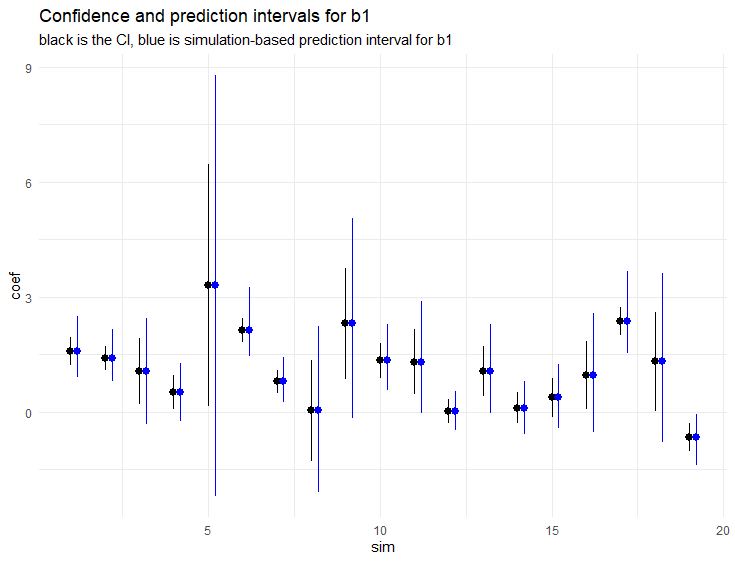
enter image description here

$\endgroup$
10
  • $\begingroup$ Prediction intervals are usually meant for the intervals around predictions rather than parameters. What do you mean here? Aren't you interested in confidence intervals? $\endgroup$
    – Tim
    Commented Feb 13, 2023 at 10:53
  • $\begingroup$ @Tim Agree that "prediction interval" might not be the best naming. The idea is this: I can make predictions for $\bar{y}$ given $\bar{x}$ - if my understanding of prediction intervals is correct, this is going the be a random vector of correlated t-distributed variables. I then should be able to transform predictions for $\bar{y}$ into predictions for some function of $\bar{y}$. $\bar{\beta}_1$ - the MLE of regression slope given $\bar{x}, \bar{y}$ is such a function. I want to construct a prediction interval for the value of this function. Does that clarify? $\endgroup$ Commented Feb 13, 2023 at 11:48
  • $\begingroup$ Could you give us an example illustrating the problem? It's not perfectly clear from your description. $\endgroup$
    – Tim
    Commented Feb 13, 2023 at 12:22
  • $\begingroup$ @Tim I added a code example showing what I am after. $\endgroup$ Commented Feb 13, 2023 at 14:07
  • 3
    $\begingroup$ Construct a pivotal quantity by dividing $\tilde\beta_1 - \hat\beta_1$ by its standard error. This involves the $x_i$'s for the new unobserved data so these must be known. Replacing $\sigma$ in the denominator by its estimate $s$ based on the observed part of the data, the resulting quantity is $t$-distributed with $n-2$ degrees of freedom, where $n$ is the sample size of the observed data. $\endgroup$ Commented Feb 13, 2023 at 15:45

1 Answer 1

2
$\begingroup$

Thanks to Jarle Tufto who provided an outline of the main idea in the comments. All errors are my own.

We can realize that if $\sigma$ was known, the distribution of the MLE of the slope is $\frac{\sigma^2}{\sum (x_i - m)^2}$ where $m$ is the observed mean of $x$ (taken from Wiki )

This means that the difference of the two MLEs is also going to be normally distributed. We however do not know $\sigma$, and plugging in the estimate of sigma from the first part, the resulting quantity is $t$-distributed with $n−2$ degrees of freedom, where $n$ is the sample size of the observed data.

So the prediction interval will be derived from t distribution centered at the MLE from the first batch of data and with standard error of $\sqrt{s^2 + \frac{\hat{\sigma}^2}{\sum (\bar{x}_i - \bar{m})^2}}$ where $\hat\sigma$ is the estimate of $\sigma$ from the first regression, $s$ is the standard error from the first regression and $\bar{m}$ is the mean of $\bar{x}$.

Adapting the code example from the question:


x <- rep(0:5, times = 4)
xbar <- rep(0:5, times = 2)

N_sims <- 10000

#Pre-allocate
y <- matrix(NA_real_, nrow = N_sims, ncol = length(x))
ybar <- matrix(NA_real_, nrow = N_sims, ncol = length(xbar))
b1 <- numeric(N_sims)
b1ci <- matrix(NA_real_, nrow = N_sims, ncol = 2)
b1bar <- numeric(N_sims)

b1pred <- matrix(NA_real_, nrow = N_sims, ncol = 2)

for(i in 1:N_sims) {
  # Choose the true values randomly
  # The results are quite similar whether I choose
  # those separately for each simulation or
  # once at the begining of the script
  true_b0 <- 1 + rnorm(1)
  true_b1 <- 0.5 + rnorm(1)
  true_sigma <- 1 + rlnorm(1)


  y_ <- rnorm(length(x), true_b0 + x * true_b1, sd = true_sigma)
  y[i,] <- y_
  fit <- lm(y_ ~ x)
  b1[i] <- coef(fit)["x"]
  b1ci[i,] <- confint(fit)["x",]

  # Calculate the prediction interval for b1bar
  b1bar_var <- sigma(fit)^2 / sum((xbar - mean(xbar))^2)
  b1_var <- vcov(fit)["x", "x"]
  diff_se <- sqrt(b1bar_var + b1_var)
  b1pred[i, ] <- b1[i] + qt(c(0.025,0.975), df = length(x) - 2) * diff_se

  ## Actually fit the new data
  ybar_ <- rnorm(length(xbar), true_b0 + xbar * true_b1, sd = true_sigma)
  ybar[i,] <- ybar_
  fitbar <- lm(ybar_ ~ xbar)
  b1bar[i] <- coef(fitbar)["xbar"]
}

cat("Coverage prediction: ", mean(b1bar >= b1pred[,1] & b1bar <= b1pred[,2]))

Shows the expected coverage behaviour.

$\endgroup$
2
  • 1
    $\begingroup$ I think there should be a square for $\hat{\sigma}$ under the square root in the equation for the standard error of the difference, right? $\endgroup$ Commented Feb 13, 2023 at 22:11
  • 1
    $\begingroup$ @COOLSerdash yes, thanks for noticing, fixed. $\endgroup$ Commented Feb 14, 2023 at 8:34

Your Answer

By clicking “Post Your Answer”, you agree to our terms of service and acknowledge you have read our privacy policy.

Not the answer you're looking for? Browse other questions tagged or ask your own question.