Linear spline and 'interaction' p value

Question

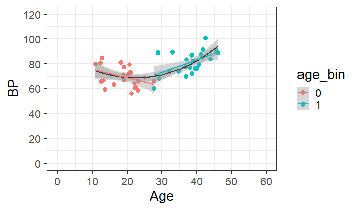
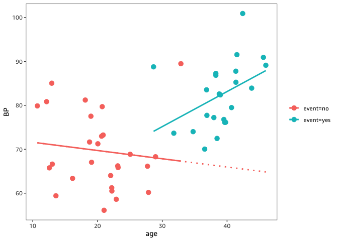
Wondering if someone can help clarify my intuition on this. Say you have a continuous covariate and a binary grouping variable and you introduce an interaction term between the two in a basic regression model (continuous outcome). Say the interaction term from the model output is not statistically significant, but suggests a 'fanning out' of the two regression slopes (the slope for one group increases at a faster rate than the slope for the second group). Would it be reasonable in this case, if one were to estimate marginal means at increasing values of the continuous covariate, that the contrast of those means may become statistically significant at some point? (or am I indeed misunderstanding some very basic concepts here).

The reason I ask is that I helped with an 'inflection-point' (linear spline) analysis. i.e. created a change-in-slope variable equal to zero below the hypothesised inflection point or the variable minus the inflection point for values above this (fairly standard change-in-slope coding). I then ran a model with both the original covariate and the change-in-slope variable together. The coefficient for the original covariate giving the slope until the inflection point and the other giving the change in slope thereafter. In a sense I consider this an interaction term.

The aim of this analysis was to see what 'effect' a particular life event had on an outcome (so in a sense a longitudinal analysis whereby the main covariate is a measure of time). After the model I used emmeans to estimate the difference in the model predicted outcome at specified time points, under the actual scenario that the life event changed the trajectory of the outcome, vs the counterfactual/hypothetical scenario that the trajectory prior to the life event was allowed to continue.

The slopes fan out, but no matter what post life-event time I estimate marginal means at, the p values remain the same as that of the model interaction. Is this just due to the way the model is parameterised? I'd like a better understanding of why.

P.S. I can try and provide some dummy data as an example if that would be helpful...

edit - 10/03/2023 I am adding some code to produce some dummy data relating to this question to hopefully assist in clarifying the question.

library(simstudy)
library(tidyverse)
library(ggplot2)
library(emmeans)

rm(list = ls())
# The following code creates some fake data for an interaction effect between a continuous (age) and binary (sex) variable on a continuous outcome (BP)
set.seed(581345)
def <- defData(varname = "male", dist = "binary", formula = .5 , id = "cid")
def <- defData(def, varname = "age", dist = "normal", formula = "20 + 20*male", variance = 20) # make males 10 yrs older on average
def <- defData(def, varname = "BP", dist = "normal", formula = "70 + 0.9*male*(age-25)", variance = 50) # make males BP 0.9 times their (age-25) higher on average
dtstudy <- genData(50, def)
dtstudy$male <- factor(dtstudy$male)

# Plot
ggplot(data = dtstudy, aes(x = age, y = BP, group = male)) +
  geom_point(aes(color = male), size = 3, position = position_jitter(w = 0.2)) +
  geom_smooth(aes(color = male), method = "lm", linewidth = 1, fullrange = F, se = F) +
  theme_bw(base_size = 20) +
  xlab("Age") + ylab("BP") +
  guides(color = guide_legend(title = "Male")) +
  scale_x_continuous(breaks = seq(0,60,10), limits = c(0,60)) +
  scale_y_continuous(breaks = seq(0,120,20), limits = c(0,120))

# Model
mod <- lm(BP ~ male * age, data = dtstudy)
summary(mod)
# Marginal Means
(emms <- emmeans(mod, ~ male + age, at = list(age = c(0, 1, 20, 40, 60, 61))))
custom <- list(`Sex diff at age = 0` = c(-1,1,0,0,0,0,0,0,0,0,0,0),
               `Sex diff at age = 1` = c(0,0,-1,1,0,0,0,0,0,0,0,0),
               `Sex diff at age = 20` = c(0,0,0,0,-1,1,0,0,0,0,0,0),
               `Sex diff at age = 40` = c(0,0,0,0,0,0,-1,1,0,0,0,0),
               `Sex diff at age = 60` = c(0,0,0,0,0,0,0,0,-1,1,0,0),
               `Sex diff at age = 61` = c(0,0,0,0,0,0,0,0,0,0,-1,1))
contrast(emms, custom) |> 
  summary(infer = T)
# While the interaction from the model is not statistically significant, contrasts of the average difference in the outcome do become statistically significant.

# But the interaction effect is really the diff in diffs 
# Diff from age = 0 to age = 1
`Sex diff at age = 0` = c(-1,1,0,0,0,0,0,0,0,0,0,0)
`Sex diff at age = 1` = c(0,0,-1,1,0,0,0,0,0,0,0,0)
contrast(emms, method = list(`Sex diff age 1 - age 0` = `Sex diff at age = 1`-`Sex diff at age = 0`))
# Diff from age = 60 to age = 61
`Sex diff at age = 60` = c(0,0,0,0,0,0,0,0,-1,1,0,0)
`Sex diff at age = 61` = c(0,0,0,0,0,0,0,0,0,0,-1,1)
contrast(emms, method = list(`Sex diff age 61 - age 60` = `Sex diff at age = 61`-`Sex diff at age = 60`))
# Diff from age = 0 to age = 60
`Sex diff at age = 0` = c(-1,1,0,0,0,0,0,0,0,0,0,0)
`Sex diff at age = 60` = c(0,0,0,0,0,0,0,0,-1,1,0,0)
contrast(emms, method = list(`Sex diff age 60 - age 0` = `Sex diff at age = 60`-`Sex diff at age = 0`))
# So the p value for the interaction remains the same no matter what diff in diff we take.

#+++++++++++++++++++++++++++++++++++++++++++++++++++++++++++++++++++++++++++++

# Now lets ignore sex completely and using the same data imagine there is an obvious change in slope at about 25 years because there has been some hypothetical life event that occurs in all 25 year olds 
# Plot
ggplot(data = dtstudy, aes(x = age, y = BP)) +
  geom_point(color = "cornflowerblue", size = 3, position = position_jitter(w = 0.2)) +
  geom_smooth(color = "cornflowerblue", method = "loess", linewidth = 1, fullrange = F, se = F) +
  theme_bw(base_size = 20) +
  xlab("Age") + ylab("BP") +
  scale_x_continuous(breaks = seq(0,60,10), limits = c(0,60)) +
  scale_y_continuous(breaks = seq(0,120,20), limits = c(0,120))

# So we create a change-in-slope variable (linear spline) to model this
dtstudy <- dtstudy |> 
  mutate(age_slope_change = ifelse(age <= 25, 0, age - 25))

# Model
mod2 <- lm(BP ~ age + age_slope_change, data = dtstudy)
summary(mod2)

# Plot
# The red line represents the counterfactual slope, had the life-event not occurred
dtstudy$pred <- predict(mod2) 
ggplot(data = dtstudy, aes(x = age, y = BP)) +
  geom_point(color = "cornflowerblue", size = 3, position = position_jitter(w = 0.2)) +
  geom_line(aes(x = age, y = pred), linewidth = 1, color = "cornflowerblue") +
  geom_segment(aes(x = 25, xend = 45, 
                   y = coef(mod2)[1] + coef(mod2)[2] * 25, 
                   yend = coef(mod2)[1] + coef(mod2)[2] * 45), 
               linewidth = 1, color = "red", linetype = "dashed") +
  theme_bw(base_size = 20) +
  xlab("Age") + ylab("BP") +
  scale_x_continuous(breaks = seq(0,60,10), limits = c(0,60)) +
  scale_y_continuous(breaks = seq(0,120,20), limits = c(0,120))

# Diff in BP between actual and counterfactual BP at age = 30 years
(emms2 <- emmeans(mod2, ~ age + age_slope_change, at = list(age = c(30), age_slope_change = c(0,5)))) |> 
  summary(infer = T)
emms2 |> 
  pairs(reverse = T)
# Diff in BP between actual and counterfactual BP at age = 40 years
(emms2 <- emmeans(mod2, ~ age + age_slope_change, at = list(age = c(40), age_slope_change = c(0,15)))) |> 
  summary(infer = T)
emms2 |> 
  pairs(reverse = T)
# So these are really just estimating interaction effects at whatever age we choose? The p value is the interaction p value.
# Is there a way to setup emmeans to calculate contrasts as in lines 28-37 above? I am guessing not as there is no corresponding factor variable in the model - the interaction is all we can calculate...

Answer 1

I think you're just accidentally confusing yourself by using slightly different methods. To answer your question - yes, in an interaction, if you compare the marginal means at different values (also called the 'pick-a-point' approach), you will eventually reach a point where there's significance (though you may be at a point beyond where your data actually go!). The common alternative is the Johnson-Neyman approach (with multiple comparison correction), which gives you the range of values over which the marginal means are significantly different.

Now, I'm just going to repeat your inflection point analysis using a slightly different approach:

## Use the chngpt library to fins the inflection point

    > library(chngpt)
> fit1=chngpt::chngptm (formula.1=BP~1, formula.2=~age, data = dtstudy, type="M01", ncpus = 1,
+                       family="gaussian")
> summary(fit1)
Change point model threshold.type:  hinge 

Coefficients:
                    est Std. Error*     (lower    upper)   p.value*
(Intercept)   69.531116    1.780648 66.0708537 73.050993 0.00000000
(age-chngpt)+  1.118825    0.497638  0.6927669  2.643508 0.02455891

Threshold:
       est Std. Error     (lower     upper) 
 27.711777   3.655929  22.217950  36.549191 
> 
> # Inflection point is at age = 27.7
> # create a new dummy variable that splits age at the inflection point
> 
> dtstudy$age_bin = 0
> dtstudy$age_bin[dtstudy$age>fit1$coefficients[3]] = 1
> dtstudy$age_bin = as.factor(dtstudy$age_bin)
> 
> # plot the result
> 
> ggplot(data = dtstudy, aes(x = age, y = BP,color =age_bin )) +
+   geom_point( size = 3, position = position_jitter(w = 0.2)) +
+   geom_smooth(inherit.aes = F,aes(x = age, y = BP),color="black", method='lm',formula ='y ~ poly(x,2)') +
+   
+   geom_smooth(aes(x = age, y = BP), method='lm',formula ='y ~ x') +
+   
+   theme_bw(base_size = 20) +
+   xlab("Age") + ylab("BP") +
+   scale_x_continuous(breaks = seq(0,60,10), limits = c(0,60)) +
+   scale_y_continuous(breaks = seq(0,120,20), limits = c(0,120))
> 

> 
> # repeat the marginal means analysis - we eventually reach significance
> 
> mod2 = lm(BP ~ age * age_bin,data=dtstudy)
> summary(mod2)

Call:
lm(formula = BP ~ age * age_bin, data = dtstudy)

Residuals:
     Min       1Q   Median       3Q      Max 
-13.6644  -5.9880  -0.2751   4.7991  17.0088 

Coefficients:
             Estimate Std. Error t value Pr(>|t|)    
(Intercept)   82.4360     6.7773  12.164 5.63e-16 ***
age           -0.6893     0.3461  -1.991 0.052398 .  
age_bin1     -39.8296    13.7691  -2.893 0.005818 ** 
age:age_bin1   1.7065     0.4667   3.656 0.000656 ***
---
Signif. codes:  0 ‘***’ 0.001 ‘**’ 0.01 ‘*’ 0.05 ‘.’ 0.1 ‘ ’ 1

Residual standard error: 7.538 on 46 degrees of freedom
Multiple R-squared:  0.4994,    Adjusted R-squared:  0.4668 
F-statistic:  15.3 on 3 and 46 DF,  p-value: 4.854e-07

> # Marginal Means
> (emms <- emmeans(mod, ~ male + age, at = list(age = c(0, 1, 20, 40, 60, 61))))
 male age emmean    SE df lower.CL upper.CL
 0      0   73.5  5.96 46     61.5     85.5
 1      0   51.2 17.00 46     17.0     85.4
 0      1   73.3  5.69 46     61.8     84.7
 1      1   52.0 16.57 46     18.7     85.4
 0     20   69.7  1.55 46     66.6     72.8
 1     20   67.2  8.42 46     50.2     84.1
 0     40   66.0  5.81 46     54.3     77.7
 1     40   83.1  1.73 46     79.7     86.6
 0     60   62.2 11.39 46     39.3     85.1
 1     60   99.1  9.24 46     80.5    117.7
 0     61   62.0 11.67 46     38.5     85.5
 1     61   99.9  9.67 46     80.4    119.3

Confidence level used: 0.95 
> custom <- list(`Sex diff at age = 0` = c(-1,1,0,0,0,0,0,0,0,0,0,0),
+                `Sex diff at age = 1` = c(0,0,-1,1,0,0,0,0,0,0,0,0),
+                `Sex diff at age = 20` = c(0,0,0,0,-1,1,0,0,0,0,0,0),
+                `Sex diff at age = 40` = c(0,0,0,0,0,0,-1,1,0,0,0,0),
+                `Sex diff at age = 60` = c(0,0,0,0,0,0,0,0,-1,1,0,0),
+                `Sex diff at age = 61` = c(0,0,0,0,0,0,0,0,0,0,-1,1))
> contrast(emms, custom) |> 
+   summary(infer = T)
 contrast             estimate    SE df lower.CL upper.CL t.ratio p.value
 Sex diff at age = 0    -22.25 18.02 46   -58.52     14.0  -1.235  0.2231
 Sex diff at age = 1    -21.27 17.52 46   -56.53     14.0  -1.214  0.2310
 Sex diff at age = 20    -2.54  8.56 46   -19.77     14.7  -0.297  0.7681
 Sex diff at age = 40    17.17  6.06 46     4.97     29.4   2.832  0.0068
 Sex diff at age = 60    36.88 14.66 46     7.37     66.4   2.515  0.0155
 Sex diff at age = 61    37.87 15.15 46     7.37     68.4   2.499  0.0161

Confidence level used: 0.95 
> 

Edit To answer a follow-up question - aren't the interaction and linear-spline models essentially identical? They are similar, but the linear-spline is missing a key piece. The linear-spline term, called age_slope_change in the original question, is equivalent to an interaction between age_bin and age (after centering age on the inflection point). Recall that an interaction model is generally of the form:

$Y = \beta _1X + \beta _2M +\beta _3XM + \epsilon$

This makes it clear that what is missing from the linear spline model is the term $\beta _2M$ - i.e., age_bin. That is, it does not model differences in the average outcome between the two groups. So if your question is "Does the slope change after the inflection point?" then the linear spline model is actually prone to false-positives!

Answer 2

This question proposes two different problems/models.

• Model A for a continuous outcome Y in two groups (men and women) with age as a covariate. Each group has its own intercept and slope (ie. group interacts with age) and we can compare the two groups at different ages.
• Model B for a continuous outcome Y as a linear function of age with a change point at age = 25 (ie. a linear spline with a knot at 25). The change point represents a life event experienced by every subject and we can compare the outcome before and after the event.

Neither model can satisfactorily answer the main question posed by the OP:

Estimate difference in the predicted outcome at specified time points, under the actual scenario that the life event changed the trajectory of the outcome, vs the counterfactual/hypothetical scenario that the trajectory prior to the life event was allowed to continue.

The models don't have a satisfactory answer because the question (as formulated here) doesn't quite make sense. If everyone experienced the life event by the age of 30, then the comparison between people who have and who haven't experienced it at the age of 60 is not a counterfactual^٭ scenario, it's an impossible scenario.

Model B cannot represent the alternative of not undergoing the life event altogether: given a specific age, model B makes an "age-appropriate" estimate E{Y | age} but there is only one possible estimate.

Model A can represent the counterfactual if we code subjects who have experienced the life event and those who haven't as different groups. Then, given any age, the model can estimate E{Y | age, event=yes} and E{Y | age, event=no}. The issue is that since everyone actually undergoes the event at a similar age, there is no overlap in age between the two groups. All comparisons between those who have and those who haven't experienced the event but are otherwise the same age require linear extrapolation. This is a huge assumption which we can never check because everyone experiences the life event.

On the plus side, once we have fitted model A, it's straightforward to compute counterfactual comparisons with emmeans. The important question is: Do these contrasts say anything meaningful?

٭ A counterfactual is the change an individual is expected to experience if they are given, say, a novel treatment vs the standard treatment. It's possible for the patient to take either the new or the current treatment; we want to know which one is expected to be more effective for the patient.

mod <- lm(BP ~ group * age, data = dtstudy)
emm <- emmeans(
  mod, ~ group | age,
  at = list(age = c(30, 40, 50, 60))
)
pairs(emm)
#> age = 30:
#>  contrast             estimate   SE df t.ratio p.value
#>  event=no - event=yes    -7.32 5.31 46  -1.378  0.1748
#> 
#> age = 35:
#>  contrast             estimate   SE df t.ratio p.value
#>  event=no - event=yes   -12.24 5.08 46  -2.413  0.0199
#> 
#> age = 40:
#>  contrast             estimate   SE df t.ratio p.value
#>  event=no - event=yes   -17.17 6.06 46  -2.832  0.0068
#> 
#> age = 50:
#>  contrast             estimate   SE df t.ratio p.value
#>  event=no - event=yes   -27.03 9.95 46  -2.716  0.0093