Estimating the probability of success in a sequence of Bernoulli Trials when the probability is changing over time

Question

Say I have a time series X from Bernoulli Trials with outcomes 0 or 1 where X(n) is the $n$th outcome in the time series. The process is driven by some probability of success $\pi$ but this probability may change over time, meaning that we have $\pi(n)$ being the probability of success of the $n$th trial. What I would like to do is to from X estimate $\pi$ at every point in some maximum likelihood sense so we could see it's evolution over time.

I would of course like $\pi$ to behave nicely as well. $\pi$ may change gradually over time but shouldn't jump erratically, the naive solution to the above I guess would have $\pi$ jumping from 0 to 1 constantly without taking the history into account which is not what we want. Would we need to prescribe some dynamics to $\pi$ itself to accomplish this?

My best guess is I should be using some Bayesian inference to accomplish this and having the prior distribution of $\pi(n)$ be centered around $\pi(n-1)$ (normally distributed probably) and updating our belief about the current value from the $n$th outcome, but I'm not sure exactly how to go about it or if this is the right approach. Would appreciate any ideas.

EDIT: I've tried to do this with Bayesian inference where I start with a prior distribution of $\pi$ and update it with one data point at a time but I'm not convinced this is exactly what I want. One issue is that it's not quite as responsive to changes in the underlying probability as I would like (from simulated data with known probability) and the credible region (width indicated by red line) is always decreasing with additional data, ideally I would like that to be able to widen in the case that the underlying probability looks like it has changed to represent that we are again in unknown territory.

import pandas as pd
import numpy as np
from scipy.stats import beta

##Bayesian with equal weights.

# Load data
p_true = np.concatenate((0.1 * np.ones(2000), 0.2 * np.ones(2000), 0.3 * np.ones(2000)))
data = np.random.binomial(n=1, p=p_true)

# Set prior parameters
mean = 0.2
alpha_prior, beta_prior = Beta_Dist_shapeparam_from_mean(mean)

# Create empty list to store posterior parameters
alpha_posterior = []
beta_posterior = []

# Iterate over each trial in the data
for i in range(len(data)):
    
    # Get outcome of current trial (0 or 1)
    outcome = data[i]
    
    # Compute posterior parameters using current outcome and prior parameters
    alpha_post = alpha_prior + outcome
    beta_post = beta_prior + 1 - outcome
    
    # Store posterior parameters for future use
    alpha_posterior.append(alpha_post)
    beta_posterior.append(beta_post)
    
    # Update prior parameters with posterior parameters
    alpha_prior = alpha_post
    beta_prior = beta_post

# Compute mean and standard deviation of posterior distribution for each trial
posterior_mean = np.array(alpha_posterior) / (np.array(alpha_posterior) + np.array(beta_posterior))
posterior_std = np.sqrt(np.array(alpha_posterior) * np.array(beta_posterior) / ((np.array(alpha_posterior) + np.array(beta_posterior)) ** 2 * (np.array(alpha_posterior) + np.array(beta_posterior) + 1)))

#Plot the posterior parameters

Answer 1

As a starting point, I would suggest one option might be to look at implementing a random walk prior on the log-odds of response. This might not be the best approach but it seems to align with your goals and if nothing else it may be educational and lead you to more fruitful options.

Specifically, if you are assuming discrete time $t$, evenly spaced (e.g. $t = 1, 2, 3, \dots$), then with no loss of generality, you can assume a binomial distribution at each time point:

$$ \begin{aligned} Y_t &= \mathsf{Bin}(n_t, p_t) \\ \mathsf{logit}(p_0) = \eta_0 &\sim \mathsf{Normal}(\mu_0, \sigma_0) \\ \mathsf{logit}(p_t) = \eta_t &= \eta_{t-1} + \epsilon_t , \quad t \in {1, 2 \dots} \\ \epsilon_t &\sim \mathsf{Normal}(0, \sigma_\epsilon) \\ \sigma_\epsilon &\sim \mathsf{Exponential}(1) \end{aligned} $$

where $Y_t$ denotes the number of events at time $t$ out of $n_t$ trials (for which your application would have $Y_t \in \{0, 1\}$ and $n_t = 1$, i.e. Bernoulli). The $\mu_0$ and $\sigma_0$ would be pre-specfied (fixed) based on prior knowledge and the other terms estimated.

To be clear, the first line is the likelihood and then the third line is the first order random walk with $\eta_t$ and $\sigma_\epsilon$ being the parameters of interest.

To implement this, you could use stan [https://mc-stan.org/] or similar. A very basic (and quite naive) implementation is shown below:

data {
  int N;
  int y[N];
  int n[N];
  int prior_only;
  real pri_mu;
  real pri_s;
  real pri_nu;
} 
transformed data {
}
parameters{
  real b0;
  real b;
  vector[N-1] delta;
  real<lower=0> nu;
} 
transformed parameters{
  vector[N] e;
  // resp is random walk
  e[1] = b0;
  for(i in 2:N){e[i] = e[i-1] + delta[i-1] * nu;}            
}   
model{
  target += normal_lpdf(b0 | pri_mu, pri_s);
  target += exponential_lpdf(nu | pri_nu);
  target += normal_lpdf(delta | 0, 1);
  if(!prior_only){target += binomial_logit_lpmf(y | n, e);}              
}   
generated quantities{
  vector[N] p;
  p = inv_logit(e);
}

which you can run in R with:

library("cmdstanr")
library("data.table")
library("ggplot2")

mod1 <- cmdstan_model(<filename here>)

set.seed(1)
K <- 100
epsilon <- rnorm(K-1, 0, 0.1)
eta <- numeric(K)
eta[1] <- qlogis(0.3)
for(i in 2:K){
  eta[i] = eta[i-1] + epsilon[i-1]
}
plot(1:K, (eta))
y <- rbinom(K, 50, plogis(eta))

ld <- list(N = K, y = y, n = rep(50, K),
           pri_mu = 0, pri_s = 10, pri_nu = 1, prior_only = F)

f1 <- mod1$sample(
  data = ld,
  chains = 3,iter_sampling = 2000,
  adapt_delta = 0.95,
  refresh = 0 # print update every 500 iters
)

p <- f1$draws(variables = "p", format = "matrix")
p_mu <- apply(p, 2, mean)
p_025 <- apply(p, 2, function(z)quantile(z, 0.025))
p_975 <- apply(p, 2, function(z)quantile(z, 0.975))


dfig <- data.table(p_mu, p_025, p_975,
                   p_obs = y/50,
                   p_tru = plogis(eta),
                   t = 1:K)

ggplot(dfig, aes(x = t, y = p_mu)) +
  geom_ribbon(aes(ymin = p_025, ymax = p_975), alpha = 0.2) +
  geom_line() +
  geom_point(aes(y = p_obs), col = 2) +
  geom_line(aes(y = p_tru), linewidth = 0.4, lty = 2)

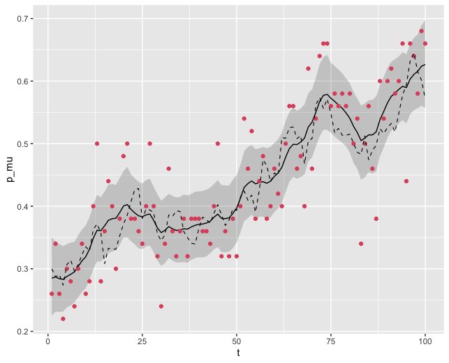
The above will begin to suffer with large numbers of observations and so may not be suitable for large datasets. In these cases, you might want to opt for an alternative, such as a penalised-spline or GP approximation (a GP will suffer with large numbers of observations due to the operations that have to be done on the covariance). The figure shows the inferred probability of response (black line) with the observed data shown as a red points and the underlying true probability of response shown as black dashed line.

The prior serves as a smoother and if this was insufficiently smooth then you could perhaps consider a second order random walk. Other considerations may relate to whether a drift component is warranted, which it might be by the sounds of your description. I will leave those for you to look into, should you wish.