Bias-Variance tradeoff in prediction versus causal inference

Question

In prediction, accepting a little more bias in exchange for a lot less variance is the very name of the game - we'll chose the model with minimal test MSE without regard for its composition (bias squared versus variance). In causal inference, we rarely - if ever - are willing to make this tradeoff. The emphasis/weight placed in textbooks preoccupied with causal inference (e.g. statistics, econometrics) on theorems such as Gauss-Markov or Cramer-Rao seems to support this point. Take for example this sentence from Peter Kennedy's A Guide to Econometrics - "In practice, the MSE criterion is not usually adopted unless the best unbiased criterion is unable to produce estimates with small variances. The problem of multicollinearity, discussed in chapter 11, is an example of such a situation." In causal inference, is an unbiased estimator with minimal variance the holy grail? Or is that just the starting point in our search? When are we willing to accept a little more bias in exchange for a lot less variance in causal inference?

In machine learning a lot of time is spent on choosing amongst models (e.g. Nearest Neighbor Model versus Linear Regression Model) and less time on choosing the estimator given a model; in statistics/econometrics - causal inference - it seems that less time is spent on choosing the statistical model (e.g. Linear Regression Model) and more time is spent on choosing the best estimator (e.g. Least Squares versus Maximum Likelihood) given a statistical model and a causal model that we have in mind. That distinction seems very relevant here and I would love it if the answer to this question would address that directly. If I made some incorrect statements in asking this question, please correct me; there are clearly some gaps in my understanding of how these topics interrelate.

Answer 1

Estimators should be judged as normal (so biased estimators are not ruled out), but with appropriate experimental protocols to deal with causality

I disagree with some of the other answers here. When conducting causal analysis, there is still a distinction between attempting to make inferences about unknown parameters, and attempting to make predictions for new instances of data (presumably subject to some intervention, since this is causal analysis). This means that we could be conducting causal inference or we could be attempting to predict new outcomes, taking account of causality. In either case, I see no particular reason why we would restrict ourselves to unbiased estimators/predictors, particularly if there are superior estimators/predictors with some bias but much better MSE (or other properties that make them superior estimators). Texts in econometrics include discussion of unbiased estimators and MVUEs, etc., for the same reason that standard statistics books include these --- because they are useful parts of estimation theory. That does not mean that they are the only admissible estimators, nor that causal analysis has some special requirement to restrict to these estimators.

When undertaking causal analysis, the only real difference to regular (non-intervention based) statistical analysis is that we make an effort to make inferences about causal effects that account for the underlying causal structure of the problem (e.g., colliders, confounding, etc.) and we impose additional experimental protocols to sever certain problematic causal effects that might exist (e.g., confounding) to allow us to interpret statistical associations as causal effects. Aside from that, all of the standard distinctions and principles of statistics apply to the estimation of the underlying model from the data. An unbiased estimator is not always a superior estimator, and when you compare it to a estimator with small bias but much smaller MSE, the unbiased estimator will usually be further away from the true parameter of interest (i.e., it will usually have more error). There may be cases when an available unbiased estimator has poor performance (e.g., high MSE) but another available biased estimator has good performance (e.g., low bias, low MSE), but to be clear, neither do we need to choose the estimator with minimum MSE; all estimators should be on the table and should be considered based on the totality of their properties and relevant trade-offs.

On this matter, it is also notable that if biased estimation were ruled inadmissible in causal analysis, this would effectively rule out Bayesian methods in this field. Bayesian estimators are almost always biased, due to the incorporation of prior information. Nevertheless, Bayesian models are known to have many good estimation properties --- their estimators are admissible, consistent (under correct model specification), and they incorporate prior information according to the principles of probability. Estimators from Bayesian analysis (e.g., the posterior mode) may have superior performance to unbiased estimators in various circumstances.

Answer 2

Adding to the response of @elbord77 -- as a statistician who has worked in public health and the insurance industry, an unbiased, imprecise estimate of a causal effect is usually preferred to a biased, precise estimate.

It comes down to whether you'd:

1. State the effect of an intervention or treatment is inconclusive and more data collection is warranted, or

2. Report with conviction ($p$-value < .05) the intervention had a positive or negative effect - however the treatment effect estimate may be biased.

Bearing in mind:

1. The intervention may have a profound impact on people's lives, and

2. Treatment effects in public health are often quite small and could be concealed by model bias.

Answer 3

In causal inference, we are usually interested in the causal effect of interventions for the purpose of informing policy decisions. Therefore, we need to estimate these causal effects without bias and in a practically useful and interpretable manner.

Regarding the bias-variance trade-off, we are usually willing to sacrifice precision in my experience because policy decisions that affect public health, for example, are often based on a meta-analysis or synthesis of multiple evidence sources, not just one. In observational studies with confounding adjustment based on models, confidence intervals are not very meaningful to begin with. Nonetheless, even for causal inference, as long as it can be justified based on domain knowledge or sensitivity analysis that the magnitude of any residual bias is small, we are often willing to make the trade off to get more precise estimates.

Because causal effects need to be interpretable and transparent to have any practical value for policy-makers, we will often use parametric models to model them. Recently, semi-parametric models are being used such that the causal effect itself is modelled parametrically for ease of interpretation but machine learning models are used to model nuisance parameters (e.g. high dimensional confounders) non-parametrically. You mention estimators: In my experience, the choice of estimators or methods has depended more on how comfortable various stakeholders are with different ones and choosing the one that everyone currently prefers rather than any principled consideration of measures such as efficiency.

Answer 4

Causal inference aims to find a model with optimal worst-case performance, so there will always be models preferrable to a biased model

When performing causal inference, there are two sources of bias:

1. Bias due to misspecification of the causal estimand
2. Bias as a property of the estimator in the sense of the bias-variance trade-off

Although both ultimately lead to biased estimates, they are conceptually different. One of the primary tasks of causal inference is to translate a causal estimand into statistical estimands that can be estimated from the data available. As such, the core of causal inference is about arriving at a suitable statistical estimand (avoiding the first type of bias), which explains why properties of the estimator (including the second type of bias) are not as central to the discussion in causal inference as they may be in other settings.

The task of causal inference can also be expressed as finding a prediction rule that is invariant to interventions on the independent variable (this idea features prominently in the ICP method). We can thus understand causal inference as a prediction problem in which we want to minimize the maximum error for any value imposed on the predictor (the connection between minimax solutions in distribution generalization and causal inference is explained for example in this paper). This means in particular that we need to make strong assumptions about the functional form of the relationship, because if the extrapolation is not clear, there is no chance of limiting the maximum error. This is a primary motivation for the common use of the linearity assumption in causal inference. Causal inference therefore assumes that the model is correctly specified and does not tolerate any bias since this would break the idea of worst-case optimality. This is why, from a strictly causal point of view, admitting any bias goes against the very goal of the inquiry. For this reason, and because of the strong assumptions on the functional form of the data generating process, trading off bias against variance as is done for prediction tasks is not the "name of the game" in causal inference.

Finally, I should say that this is the theoretical view, and in practice things may look quite different. In the real-world, interventions are often confined to a certain range and I'm sure the idea of trading off bias and variance in causal inference may not seem so foreign to a practitioner and may in fact be necessitated by imperfect knowledge of the underlying data generating process.

Answer 5

I'm $100\%$ with Ben. I have seen an obsession with unbiased estimators in causal inference and not understood it. After all, we're drawing our causal inferences based on the parameters, and we use statistical inference to guess what the parameter values are. If we have an estimated value of the parameter that is off by a large amount (which can happen for an unbiased estimator with high variance, see the graph below), we might make an incorrect conclusion, perhaps even get the incorrect sign!

The sentiment almost seems to be that estimating using an unbiased estimator gives the true parameter value, and it simply does not, and the amount by which our estimated value is misses the true value could be considerable if we do not have a good control of the variance. A biased estimator can be off by a bit in expectation, sure, yet put us in position not to deviate very far from the true value. For a true parameter value of zero, consider the two densities below, one of which is the density of a possible unbiased estimator and the other of which is the density of a possible biased estimator with much lower variance and mean squared error. The unbiased estimator has so much higher of a probability of being far away from the true value!

library(ggplot2)
set.seed(2023)
s <- seq(-1.5, 1.5, 0.01)
y1 <- dnorm(s, 0.1, 0.1)
y2 <- dnorm(s, 0, 0.5)
# y1 <- y1/max(y1, y2) # Uncomment these lines to scale the densities, as I first did
# y2 <- y2/max(y1, y2) # Uncomment these lines to scale the densities, as I first did
d1 <- data.frame(
  Estimate = s,
  Density = y1,
  Estimator = "Biased"
)
d2 <- data.frame(
  Estimate = s,
  Density = y2,
  Estimator = "Unbiased"
)
df_plot <- rbind(d1, d2)
ggplot(df_plot, aes(x = Estimate, y = Density, col = Estimator)) +
  geom_line() +
  theme(
    legend.position = "bottom",  
    legend.key.width = unit(2.5, "cm")
  )

Answer 6

The focus on ``unbiasedness'' in causal inference arises from different considerations. The purpose of this comment to clarify why this is and show how it sheds lights on the role of classical statistical optimality.

Setup

Consider observed data from a distribution $\mathbb{P}_0$ from which there are $n$ i.i.d draws with empirical distribution $\mathbb{P}_n$. A typical statistical problem involves constructing an estimator from $\mathbb{P}_n$ to estimate a summary of $\mathbb{P}_0$. Causal inference is different.

Consider an alternative distribution $\mathbb{P}_0^*$ of the observed data, and suppose the estimand $\psi_1(\mathbb{P}_0^*)$ is a summary of $\mathbb{P}_0^*$. The fundamental estimation problem in causal inference is to determine an estimator $\psi_2(\mathbb{P}_n)$ that should be as close as possible to the estimand. Since the empirical distribution $\mathbb{P}_n$ is based on draws from $\mathbb{P}_0$ rather than the alternative distribution $\mathbb{P}_0^*$, this problem is fundamentally different than a typical statistical problem.

Identification

For a reader, please consider how you would approach such a problem. I don't think it is at all clear. In fact, it may seem impossible: there's no way rub the data in $\mathbb{P}_n$ together to learn about the arbitrary distribution $\mathbb{P}_0^*$. This is true, so causal inference starts off assuming there's a relationship between $\mathbb{P}_0$ and $\mathbb{P}_0^*$. Examples include assuming there are no unmeasured confounders, an instrument is available, etc.

Identification is the result of determining some $\psi_3$ so that $\psi_1(\mathbb{P}_0^*)=\psi_3(\mathbb{P}_0)$. In this case the estimand is a summary of the true distribution $\mathbb{P}_0$ that we learn about with our sample $\mathbb{P}_n$. As sometimes said, the latter is ``unbiased'' for the former.

Estimation

Suppose that the estimand was identified so that there exists some $\psi_3$. The fundamental estimation problem in causal inference is thus to determine an estimator $\psi_2(\mathbb{P}_n)$ that should be as close as possible to $\psi_3(\mathbb{P}_0)$. This is now a traditional statistical problem! The considerations from the others' posts concerning bias-variance tradeoffs now apply---after identification.

Answer 7

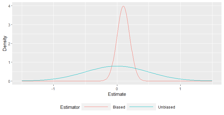
Some notes on the mater, coming from econometrics:

After the advances in computing power made Monte Carlo simulations easy, it has become standard to assess finite-sample properties of estimators through such simulations (since their finite-sample distribution is almost always unknown). And in them, casual observation indicates that almost always the Mean Squared Error (MSE) or Root Mean Squared Error (RMSE) criterion is used to assess performance, stand-alone or in comparison... so it would appear that academic econometrics at least have embraced the ``bias-variance" trade-off, since we can get better MSE, with a succesful such trade-off... Is that ok?

We should ask ourselves

Q: When MSE is a reasonable criterion to apply in order to assess the performance of an estimator?

A: when our goal is to construct an estimator to be used repeatedly as a prediction/forecasting tool. Think macroeconomic models for government policy or big-business planning, think large-scale factory production. In such situations, what is our prediction error ``on average" does matter as regards the overall costs of inaccuracy.

But in very many cases of applied econometric research, the goal is not to predict the dependent variable, but to measure regressor effects on the dependent variable after the fact, to uncover what has happened. This will certainly inform future decisions in comparable situations, but not in the same way as mentioned just above. Here, I argue that it is more pertinent and more useful to be able to determine the range of values that the unknown effect is likely to have taken, given your estimate. This points towards the construction of confidence intervals (CI) around the estimate, and the measurement of the``coverage probability": what is the percentage of times the true value of the unknown effect falls inside the constructed confidence interval.

Obviously, we would want to have a CI as short as possible with a coverage probability as high as possible... (and I always talk about the empirical properties of the CI, not the theoretical ones if the distribution used to construct it happens to be exactly what holds in the data).

Focusing on the case where we treat our estimator as having a Normal distribution (which is what we do most of the times relying on asymptotics), I will show next that

Claim 1. The introduction of any bias keeping the variance unchanged reduces the coverage probability, without shortening the CI.

Claim 2. A successful "bias-variance trade-off" reduces the coverage probability even more - but at least here, we get a shorter CI. So the bias-variance trade-off creates another trade-off: the "length-coverage" one.

Claim 3. For small relative bias, the reduction in coverage probability appears tolerable, against the magnitude of the benefit of a shorter CI.

Let $\beta$ be the unknown effect (say, a coefficient), and $b$ its estimator with standard deviation $\sigma$. We treat $b$ as Normal, and we allow for the possibility of (positive or negative) bias $B$ (which we do not know if it exists). Then

$$\frac{b-\beta}{\sigma} \sim {\rm N}\left(\frac {B}{\sigma}, 1\right).$$ In fact we will define $\xi \equiv |B/\sigma|$ and $s\equiv {\rm sgn}(\xi)\in \{-1,0,1\}$, and so $$\frac{b-\beta}{\sigma} \sim {\rm N}\left(s\xi, 1\right).$$

A typical CI is constructed as $[b \pm\sigma z_{\alpha/2}]$, where $z_{\alpha/2}$ is the $\alpha/2$-quantile of the Normal distribution.

We want the coverage probability ${\rm CP}$, which is the probability of the event $$\Big\{b -\sigma z_{\alpha/2} \leq \beta \leq b +\sigma z_{\alpha/2}\Big\}$$ which after standard manipualtions gives

$${\rm CP} = \Pr\left(-z_{\alpha/2} \leq \frac{b-\beta}{\sigma} \leq z_{\alpha/2}\right).$$

Taking into account the possibility of bias, and the Normality of our estimator, this is, for $\Phi$ the standard Normal CDF, $${\rm CP} = \Phi\left(z_{\alpha/2}- s\xi\right) - \Phi\left(-z_{\alpha/2}- s\xi\right).$$

Consider now how the coverage probability changes with $\xi$, $\phi$ being the standard Normal density (an even function): \begin{align} \frac{\partial {\rm CP}}{\partial \xi} &= -s\phi\left(z_{\alpha/2}- s\xi\right) + s\phi\left(z_{\alpha/2}+ s\xi\right)\\ &= s\cdot \left[\phi\left(z_{\alpha/2}+ s\xi\right) - \phi\left(z_{\alpha/2}- s\xi\right)\right]\\ &=s\cdot \phi\left(z_{\alpha/2}+ s\xi\right)\left[1 - \frac{\phi\left(z_{\alpha/2}- s\xi\right)}{\phi\left(z_{\alpha/2}+ s\xi\right)}\right]\\ &=s\cdot \phi\left(z_{\alpha/2}+ s\xi\right)\left[1 - \exp\big\{2z_{\alpha/2}s\xi \big\}\right]. \end{align}

One can verify that $$\begin{cases} \xi = 0 \qquad \frac{\partial {\rm CP}}{\partial \xi} = 0\\ \\ \xi \neq 0 \qquad \frac{\partial {\rm CP}}{\partial \xi} < 0 \end{cases} $$

So the existence of bias always reduces the coverage probability, and if we managed that without reducing the variance, we are unambiguously worse-off, whether we look at MSE or the $CI$. (Claim 1.)

Consider now a successful "bias-variance trade off". This means that we have $|B|\neq 0$ and enough $\sigma \downarrow$ to reduce MSE... but this will increase $\xi$ on two counts -its numerator will increase and its denominator will decrease. So we will have larger decrease in the coverage probability, but a shorter CI (Claim 2).

As for Claim 3., what kind of bias magnitudes are we talking about here? I would say, some small percentage of the variance, otherwise I doubt anyone would accept it. So suppose we have $B^2 = 0.1\sigma^2$ and let's say we achieve a $20\%$ reduction in the variance. Our MSE was without bias $\sigma^2$ and now it becomes $${\rm MSE}|_{B} = (1-0.2)\sigma^2 + 0.1\sigma^2 = 0.9 \sigma^2 < {\rm MSE}|_{U}.$$ That's a successful bias-variance trade-off.

In this numerical example, we have $\xi = \sqrt{0.1/0.8}= 0.3535$. Let's turn now to the Coverage Probability. Suppose we want a $0.9-{\rm CI}$ so $z_{\alpha/2} = z_{0.95} = 1.645$.

Suppose the bias is positive (overestimation of $\beta$ on average, sign included). Then $${\rm CP}|_{B=0} = \Phi\left(1.645\right) - \Phi\left(-1.645\right) = 0.90.$$

$${\rm CP}(B=\sigma\sqrt{0.1},\, \sigma(B) = \sqrt{0.8}\sigma) = \Phi\left(1.645- \frac{\sqrt{0.1}}{\sqrt{0.8}}\right) - \Phi\left(-1.645- \frac{\sqrt{0.1}}{\sqrt{0.8}}\right) = 0.879.$$

This bias-variance trade-off resulted in our ${\rm CI}$ being now $1-\sqrt{0.8}=11.5\%$ shorter, while the coverage probability reduced by $2$ probability points... many people would be willing to live with this trade-off.

It is an interesting exercise to compute how the coverage probability reduces as $\xi$ increases and, for the different variance reductions that can be associated with the same $\xi$, how much the length of the CI shortens, to get a fuller quantitative picture of this ``length-coverage" trade-off.