Is it valid to calculate the AUPRC of a model by undersampling one class and then re-oversampling its results?
Yes, but only if you're careful in the implementation. Throwing re-sampled scores into scikit-learn's average_precision_score gives overestimates at ~25% relative error for your data. (Overestimation is demonstrated in the first version of this answer, which is based on this older version of the simulation code. I haven't completely ruled out that scikit-learn's AUPRC estimate on the whole sample is biased. Either way, you need to be careful in the implementation.) These issues are well-known enough that there's a paper which proposed throwing out AUPRC in favor of a different metric:
Flach, Peter, and Meelis Kull. "Precision-recall-gain curves: PR analysis done right." Advances in neural information processing systems 28 (2015).
Back to your question. Empirically, the following re-sampling-based estimators are somewhat unbiased:
$\text{repeat}$: down-sample the more prevalent class, compute predictions, then repeat them back to the original size
$\text{up-sample}$: down-sample the more prevalent class, compute predictions, then randomly up-sample them back to the original size (from @usεr11852's comment)
$\text{re-weigh}$: down-sample the more prevalent class, compute predictions, then re-weigh them in the computation of AUPRC (derived in the next section).
My implementations of the pure down-sampling estimator—
- $\text{down-sample}$: down-sample the dataset uniformly at random, paying no attention to the class
—appear to be slightly biased, but I don't know why.
Derivation of $\text{re-weigh}$ estimator
Repeating data can be codified as re-weighing in the AUPRC scoring function. So only the scoring function needs to be modified, not the data. Perhaps this fact saves you some compute for super large-scale evaluations.
Let $P$ represent the universe where data are not re-sampled. Let $Q$ represent the universe where we re-sample. In your re-sampling scheme, $P(Y = 1) = 1\text{k} / (1\text{k} + 100\text{k})$ and $Q(Y = 1) = 1/2$.
Given a threshold $t \in (0, 1)$, call $p_P(t)$ the model's precision on $P$ at $t$, call $r_P(t)$ the recall, and $f_P(t)$ the false positive rate, i.e.,
$$
\begin{equation*}
p_P(t) = P(Y = 1 \: | \: \hat{Y} > t) \\
r_P(t) = P(\hat{Y} > t \: | \: Y = 1) \\
f_P(t) = P(\hat{Y} > t \: | \: Y = 0).
\end{equation*}
$$
The AUPRC score we'd like to estimate is that on $P$ :
$$
\begin{align*}
\text{AUPRC} &= \int_{t} p_P(t) dr_P(t) \\
&\approx \sum_{i=2}^{n} p_P(t_i) (r_P(t_i) - r_P(t_{i-1})). \\
\end{align*}
$$
In the sum above, $\{t_i\}_{i=1}^{n}$ is a grid of decreasing thresholds over $(0, 1)$, which implies that $r_P(t_i)$ monotonically increases.
The game is to estimate each $p_P(t_i)$ and $r_P(t_i)$ using metrics from $Q$—the universe where it's less costly to compute model metrics. The trick is to realize that $Q$ and $P$ are equivalent when they're conditioned on the class ($Y = 0$ or $Y = 1$), because the class frequency is the only difference between $Q$ and $P$. This fact implies $r_P(t) = r_Q(t)$ and $f_P(t) = f_Q(t)$. The precision calculation requires some manipulation:
$$
\begin{align*}
p_P(t) &= \frac{r_P(t) P(Y=1)}{P(\hat{Y} > t)} && \text{Bayes' rule} \\
&= \frac{r_Q(t) P(Y=1)}{P(\hat{Y} > t)} && \text{class-conditional}
\end{align*}
$$
where
$$
\begin{align*}
P(\hat{Y} > t) &= r_P(t) P(Y=1) + f_P(t) (1 - P(Y=1)) && \text{total probability} \\
&= r_Q(t) P(Y=1) + f_Q(t) (1 - P(Y=1)) && \text{class-conditional}.
\end{align*}
$$
Plugging it back in:
$$
\begin{align*}
p_P(t) = \frac{r_Q(t) P(Y=1)}{r_Q(t) P(Y=1) + f_Q(t) (1 - P(Y=1))}
\end{align*}
$$
This proves that $P(Y=1), r_Q(t)$, and $f_Q(t)$ are sufficient to calculate $\text{AUPRC}$.
Simulations
Code for this simulation is available here.
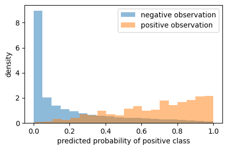
Let's empirically evaluate the AUPRC estimators on the Beta-distributed predictions from your simulation:

Repeating the estimator definitions (for easier reference):
$\text{down-sample}$: down-sample the dataset randomly
$\text{repeat}$: down-sample the more prevalent class, compute predictions, then repeat them back to the original size
$\text{up-sample}$: down-sample the more prevalent class, compute predictions, then randomly up-sample them back to the original size (from @usεr11852's comment)
- as suggested in the linked comment, the implementation of the ECDF inverse includes linear interpolation. See the
sample method in the code
$\text{re-weigh}$: down-sample the more prevalent class, compute predictions, then re-weigh them in the computation of AUPRC.
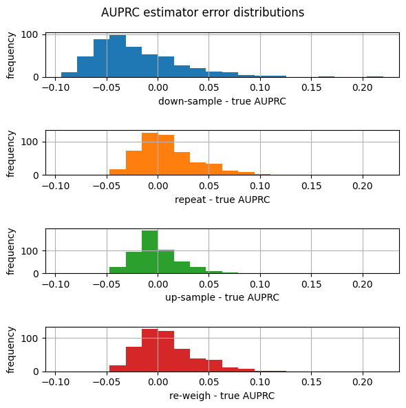
The simulation computes the signed difference between the estimator's observed AUPRC and the "true" AUPRC—that on the full dataset. Each estimator uses the same number of model() calls, i.e., the model compute is held constant.

Here are summary statistics:
       error down-sample  error repeat  error up-sample  error re-weigh
count            500.000       500.000          500.000         500.000
mean              -0.021         0.009           -0.002           0.009
std                0.041         0.027            0.020           0.027
min               -0.094        -0.042           -0.047          -0.042
25%               -0.050        -0.010           -0.015          -0.010
50%               -0.031         0.004           -0.005           0.004
75%                0.001         0.024            0.009           0.024
max                0.220         0.113            0.066           0.113
Notes:
$\text{up-sample}$ has the lowest bias and variance. It gets bonus points b/c you can repeatedly up-sample, which allows you to be transparent about the variance from up-sampling. Though there's no cheap way to convey the important source of variation—that from the initial down-sampling.
$\text{down-sample}$ has significantly higher variance than the rest because it only looks at a handful of the less prevalent class. It's also weird b/c the direction of bias depends on the implementation. The first version of my simulation demonstrates overestimation, as does your simulation. Both used scikit-learn's implementation.


