Understanding the computation of sample bias and variance

Question

I believe I am confused in some fundamental way about the bias-variance tradeoff and I am trying to clear up my confusion. Sorry for a bit of a preliminary rambling -- I wanted to put my understanding on the table.

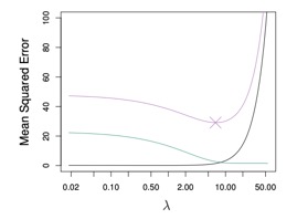
I was reading "An Introduction to Statistical Learning" and in particular I was learning about ridge regression. The following diagram is from the book to illustrate the affect of changing the tuning parameter $\lambda$ in ridge regression on the error of the model. The pink line represents the mean square error, the green line represents the variance, and the black line represents the squared bias.

In the back of my mind is the case of estimators in statistical inference where we have $$ \mathbb{E}[(\hat{\theta} - \theta)^2] = \text{bias}^2(\hat{\theta}) + \text{Var}(\hat{\theta}) $$

When dealing with samples, an analogous equation holds where we apply the usual process of replacing expected values with averages over samples.

I know that in the context of regression we have a model $Y = f(X) + \epsilon$ and we want to estimate $f$ with some $\hat{f}$ given several i.i.d. observations $X_1,...,X_n$ and $Y_1,...,Y_n$ each satisfying the same relation. We can then pick a particular pair $(x_0, y_0)$ in this setting we have $$ \mathbb{E}[(y_0 - \hat{f}(x_0))^2] = \text{bias}^2(\hat{f}(x_0)) + \text{Var}(\hat{f}(x_0)) + \text{Var}(\epsilon) $$ In this diagram, we are not seeing that the mean square error is equal to the sum of the squared bias and the variance due to this final $\text{Var}(\epsilon)$ term.

My question: how where the (sample!) mean square error, square bias, and variance likely calculated in this example?

Here is my guess:

Some point $(x_0, y_0)$ was chosen and the data was broken up and $\hat{f}$ was computed using the different pieces. Then this was used to estimate the mean square error, squared bias, and variance terms. Maybe this was actually done for many points $(x_0, y_0)$ and the results averaged. Do you think this is a reasonable guess? Is there a standard way to do this?

Answer 1

I assume you are talking about the left-hand side of Figure 6.5. Here is a link to ISL for anyone who might not have it available. (Hastie, p. 240)

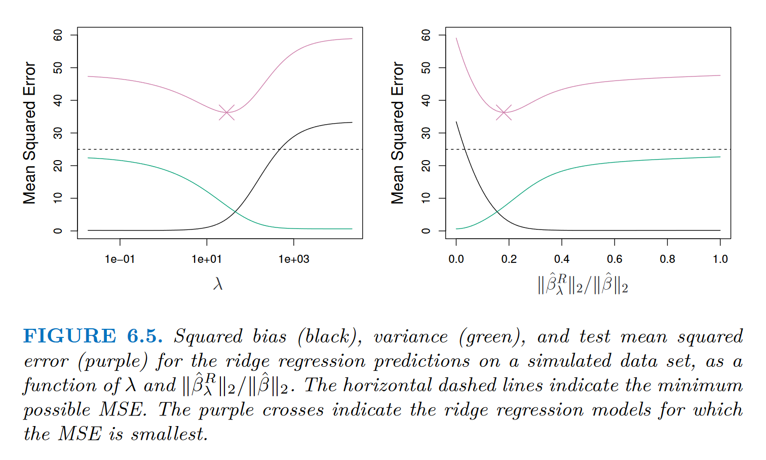
I see the graph you provide is a little bit different. I assume you tried to replicate their code? In the original image, see below, there is a dashed line that indicates the 'minimum possible MSE'.

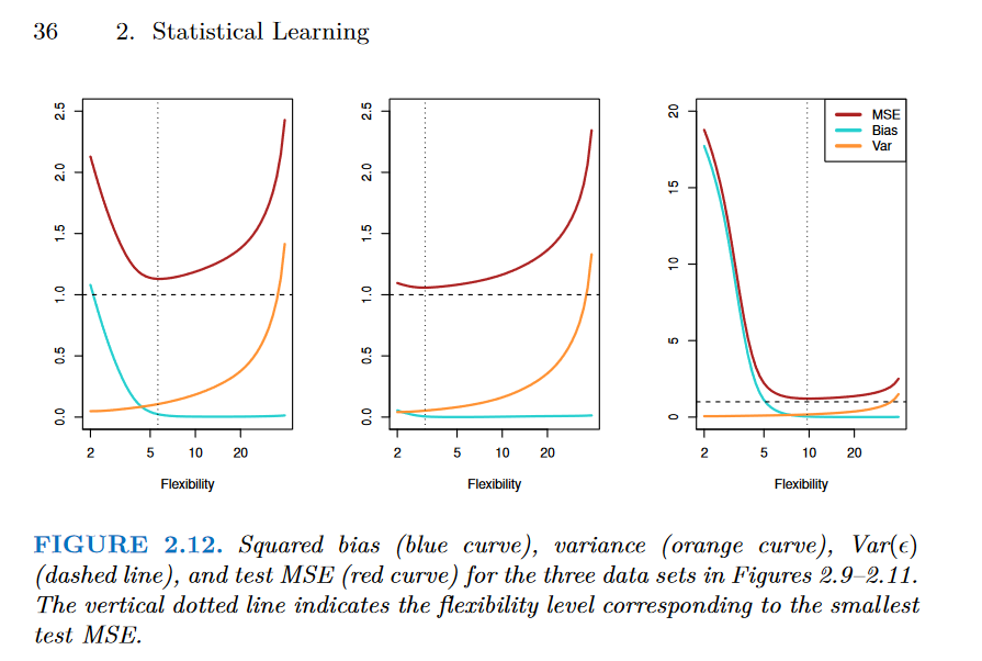
I totally understand your confusion, this is terribly worded. The dashed line is equal to $Var(\epsilon)$, what they call the irreducible error in the model (Hastie, p. 19). So, you are adding together the green, black, AND dashed lines to get the purple line. They are more clear in Figure 2.12 on page 36 (Hastie, p. 36):

I believe the crux of your confusion is that these lines being plotted are an estimation of the test data's MSE, bias, and variance (i.e. not the sample MSE, bias, and variance). Instead, it is calculated analytically using the model that was trained. These graphs are plotted so that we may see where we expect test MSE to be the lowest, so that we may pick the optimal $\lambda$ value. If we used any of the test set, we'd be peeking into the holdout test set (one of the biggest no-no's in ML)!

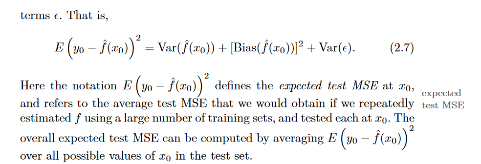
Equation 2.7 kind of addresses this, but in an obtuse and unclear way. (Hastie p. 34) Yes, technically, you can estimate the expected value of the test MSE by just calculating the sample MSE of the test set, but you would then be prohibited from varying $\lambda$.

It is important to note that $Var(\hat{f}(x_0))$ is not the variance of the actual test data, but the variance of the trained model itself, i.e. $Var(\hat{f}(x_0)) = Var(\hat{\beta}_0 + x_0\hat{\beta}_1)$, which is nontrivial to compute, especially in ridge regression. The same can be said about the bias. $x_0$ is an arbitrary test data point, which we do not know.

If you wanted to calculate the true sample MSE for the test set, you would have to do so after picking a final model via:

$$MSE = \frac 1n \sum_{k=1}^{m} (y_k-\hat{f}(x_k))^2$$

where $K$ is the set of your testing data.

Also note that $\epsilon$ is usually an assumption made by the experimenter, we do not know its true variance, but assume:

$$\epsilon_i ~iid~ \sim N(0, \sigma^2)$$

Thus $Var(\epsilon)=\sigma^2$ is constant. In the above pictures, I believe the authors chose 25 and 1, respectively.

ISL is not very transparent about how these expected values are calculated. I believe this is done on purpose, as they are kind of outside the scope of the book. Also note that the OLS solution to the regression problem is unbiased, and thus MSE is just equal to the reducible and irreducible variances. Bias is introduced via the regularization term $\lambda$, which is why regularization is important in the first place. We trade some bias for lower variance and lower MSE as a whole.

If you are still interested in the actual calculations for the expected test MSE, see equation 2.27 in ESL (Hastie p. 26). (They write 'EPE', which is expected prediction error. Earlier, they define this as the expectation of the loss function, evaluated at our estimate (aka the risk function). Under squared error loss, the risk is simply MSE.)