Discrepancy between the results of the ANOVA and the post-hoc test: How should be such results interpreted and presented?

Question

It is possible to find discrepancies between the results of ANOVA and post-hoc tests. The results of post-hoc tests are valid (with the exception of the Fisher LSD test) even if the overall P value for the ANOVA is greater than 0.05 (1, 2, 3, 4).

How should such results be presented and interpreted? There are some questions on this subject, but the answers are more or less theoretical (5, 6, 3, 4). I could not find any papers (biology, ecology and related fields) with such results.

Therefore, I would like to know how to present and interpret such results using a real example: I used a linear mixed model (function lmer, R package lme4) to analyse the effect of cover of two invasive plant species (Solidago spp.) on the diversity of invaded plant communities. The response variable is species richness, the explanatory variables are categorical - invasive species (2 levels: S. canadensis and S. gigantea), cover of invasive species (3 levels: C = ~0%, T = ~30% and D = ~80%) and their interaction.

Data

While the results of the anova (function Anova, type 3 and 2; package car) suggest no significant interaction, visual inspection of the boxplot suggests the opposite, which was confirmed by post-hoc tests (function avg_comparisons from the package marginaleffects). See below.

So how should I present and interpret these results?

(By the way, why are there no values for intercept in the type 2 Anova outputs?)

R script:

> library(lme4)
> library(car)
> library(MuMIn)
> library(marginaleffects)
> m1<-lmer(Hillall_0 ~ solidago * plot + (1 | locality), data=dat)

> Anova(m1, type="III", icontrasts=c("contr.sum", "contr.poly"))
Analysis of Deviance Table (Type III Wald chisquare tests)
Response: Hillall_0
Chisq Df Pr(>Chisq)
(Intercept)   185.7266  1  < 2.2e-16 ***
solidago        8.4379  1  0.0036749 **
plot           16.4066  2  0.0002737 ***
solidago:plot   4.7866  2  0.0913297 . 
---
Signif. codes:  0 ‘***’ 0.001 ‘**’ 0.01 ‘*’ 0.05 ‘.’ 0.1 ‘ ’ 1

> Anova(m1, type="II")
Analysis of Deviance Table (Type II Wald chisquare tests)
Response: Hillall_0
       Chisq Df Pr(>Chisq) 
solidago      14.3900  1  0.0001486 ***
plot          12.8453  2  0.0016243 ** 
solidago:plot  4.7866  2  0.0913297 . 
---
Signif. codes:  0 ‘***’ 0.001 ‘**’ 0.01 ‘*’ 0.05 ‘.’ 0.1 ‘ ’ 1

> r.squaredGLMM(m1, pj2014 = F)
       R2m       R2c
[1,] 0.3518038 0.3518038

Post-hoc tests:

> avg_comparisons(m1, variables = "solidago", by = "plot")
Term                          Contrast plot Estimate Std. Error      z Pr(>|z|)   S 2.5 % 97.5 %
solidago mean(gigantea) - mean(canadensis)    C    -12.6       4.34 -2.905  0.00367 8.1 -21.1   -4.1
solidago mean(gigantea) - mean(canadensis)    D     -1.8       4.34 -0.415  0.67816 0.6 -10.3    6.7
solidago mean(gigantea) - mean(canadensis)    T    -14.1       4.34 -3.251  0.00115 9.8 -22.6   -5.6
Columns: term, contrast, plot, estimate, std.error, statistic, p.value, s.value, conf.low, conf.high, predicted_lo, predicted_hi, predicted
Type:  response

> avg_comparisons(m1, variables = "plot", by = "solidago")
Term          Contrast   solidago Estimate Std. Error      z Pr(>|z|)    S 2.5 % 97.5 %
plot mean(D) - mean(C) canadensis    -15.6       4.34 -3.596   <0.001 11.6 -24.1   -7.1
plot mean(D) - mean(C) gigantea       -4.8       4.34 -1.107    0.268  1.9 -13.3    3.7
plot mean(T) - mean(C) canadensis     -0.8       4.34 -0.184    0.854  0.2  -9.3    7.7
plot mean(T) - mean(C) gigantea       -2.3       4.34 -0.530    0.596  0.7 -10.8    6.2
Columns: term, contrast, solidago, estimate, std.error, statistic, p.value, s.value, conf.low, conf.high, predicted_lo, predicted_hi, predicted
Type:  response

> avg_comparisons(m1, variables = "solidago", by = "plot", hypothesis = "pairwise")
Term Estimate Std. Error      z Pr(>|z|)   S   2.5 % 97.5 %
C - D    -10.8       6.13 -1.761   0.0783 3.7 -22.823   1.22
C - T      1.5       6.13  0.245   0.8068 0.3 -10.523  13.52
D - T     12.3       6.13  2.005   0.0450 4.5   0.277  24.32
Columns: term, estimate, std.error, statistic, p.value, s.value, conf.low, conf.high
Type:  response

> avg_comparisons(m1, variables = "plot", by = "solidago", hypothesis = "pairwise")
Term Estimate Std. Error      z Pr(>|z|)    S 2.5 % 97.5 %
(mean(D) - mean(C), canadensis) - (mean(D) - mean(C), gigantea)      -10.8       6.13 -1.761   0.0783  3.7 -22.8   1.22
(mean(D) - mean(C), canadensis) - (mean(T) - mean(C), canadensis)    -14.8       4.34 -3.412   <0.001 10.6 -23.3  -6.30
(mean(D) - mean(C), canadensis) - (mean(T) - mean(C), gigantea)      -13.3       6.13 -2.168   0.0301  5.1 -25.3  -1.28
(mean(D) - mean(C), gigantea) - (mean(T) - mean(C), canadensis)       -4.0       6.13 -0.652   0.5144  1.0 -16.0   8.02
(mean(D) - mean(C), gigantea) - (mean(T) - mean(C), gigantea)         -2.5       4.34 -0.576   0.5644  0.8 -11.0   6.00
(mean(T) - mean(C), canadensis) - (mean(T) - mean(C), gigantea)        1.5       6.13  0.245   0.8068  0.3 -10.5  13.52
Columns: term, estimate, std.error, statistic, p.value, s.value, conf.low, conf.high
Type:  response

Answer 1

There are two remarks with the comparison using the boxplot

Medians vs Means

Your boxplots are plotting the medians and it looks like the case of D cover has an opposite effect.

But this is not the case when you compare the means. Then you have effect sizes in the same direction.

So the plot with the medians make the differences in effect sizes appear a bit stronger.

Contrast                                 Estimate  Pr(>|z|)   
mean(gigantea) - mean(canadensis)    C  -12.6      0.00367 
mean(gigantea) - mean(canadensis)    D  -1.8       0.67816 
mean(gigantea) - mean(canadensis)    T  -14.1      0.00115 

Multiple comparisons

Still you have one effect size that is a lot different, why wouldn't this result into a significant interaction? The reason is that you have three levels which increases the odds that one of them happens to be different. Your case is a bit borderline. The result is not very significant, but neither is it insignificant. Remember that absence of statistical significance is not proof that there is no effect.

If you would compute a t-statistic out of the pairwise differences between those three effects. For example, with one of those comparisons you get an effect size difference of $$(-12.6) - (-1.8) = -10.8$$ then you get the comparisons in the lines from the final table

Term                                                                 Estimate  z        Pr(>|z|)
(mean(D) - mean(C), canadensis) - (mean(D) - mean(C), gigantea)     -10.8     -1.761    0.0783
(mean(D) - mean(C), canadensis) - (mean(T) - mean(C), gigantea)     -13.3     -2.168    0.0301 
(mean(T) - mean(C), canadensis) - (mean(T) - mean(C), gigantea)       1.5      0.245    0.8068

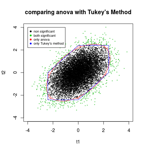
The z/t-scores of 0.245, -2.168 and -1.761 are not very large, or at the border of typically applied confidence levels. Compare with this figure from The theory behind Tukey's HSD test.

The individual comparisons can be significant at a 5% level. Like the individual z/t-score of -2.168 is described with a p-value of 0.0301, and this is what you intuitively see in the boxplots. However, when you look at multiple comparisons and wish to compensate for that, then you need to be stricter and use the blue or the red borders from the image above.