intuition linear regression stepwise selection of predictors

Question

I am using a tool in genetics, which works very similar to stepwise linear regression (its called GCTA-COJO for those interested). Essentially the starting situation looks like this:

You have 1000s of predictors (called SNP1, SNP2, ...) and a continous trait Y you want to predict. In the first step, you would fit a linear model which would only include one of the predictors (i.e. lm(Y~SNP1), lm(Y~SNP2), ...).

In the second step, you fit a joint model, which includes multiple predictors (i.e. lm(Y~SNP1+SNP5+SNP159)). Here, I noticed, that often times predictors which are not significantly associated with the outcome Y in the "single predictor" association test (i.e. lm(Y~SNP1)) become significant, when they are included in the joint model (lm(Y~SNP1+SNP5+SNP159)). Somehow, I have a very hard time understanding how such a thing is possible, and would love if somebody could give me an intuitive explaintion which this is possible.

Here is some example data, which describes my situation reasonably well:

library(broom)
library(tidyverse)

set.seed(123)  # Set seed for reproducibility

# Generate 100 observations for each variable
n <- 100

# Generate predictors with varying correlations
predictors <- matrix(rnorm(20 * n), nrow = n)
predictors[, 1:5] <- predictors[, 1] + rnorm(n, sd = 0.2)  # Introduce some correlation
predictors[, 6:10] <- predictors[, 5] + rnorm(n, sd = 0.3)  # Introduce more correlation

# Generate the outcome variable with varying relationships to predictors
Y <- 2 + 0.5 * predictors[, 1] + 0.8 * predictors[, 5] + 0.3 * predictors[, 10] + rnorm(n)

# Combine into a data frame

data <- data.frame(Y, predictors)
names(data)[-1] <- paste0("X", 1:20)  # Assign column names

# Store the names of the 20 predictors
predictors <- names(data)[-1]  # Assuming Y is the first column

# Fit individual linear regressions for each predictor
for (predictor in predictors) {
  model <- lm(formula = Y ~ data[[predictor]], data = data)
  print(predictor)
  print(tidy(model))
}

# Full model with all predictors
full_model <- lm(Y ~ ., data = data)

# Stepwise selection using AIC
best_model <- step(full_model, direction = "both")  # Consider both forward and backward selection

# Print the summary of the selected model
summary(best_model)

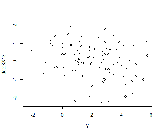
In this example, predictor13 is not significant in the single variant association test, but in the joined model (best_model), we can see that it becomes significantly associated. This is surprsing for me, given that it does not seem like there is any association between the two variables:

Any insights into why this is possible are very much appreciated!

Cheers!

Answer 1

First, your full model has huge collinearity problems:

library(olsrr)
ols_coll_diag(full_model)

reveals that the highest condition indexes are NaN, but the 17th is on the order of $10^{19}$.

Second, stepwise is a very problematic method of variable selection. Basically, all the output is wrong. p values are too low, standard errors too small, and parameter estimates biased away from zero. This has been covered here many times.

Finally, to answer your question (and with all that said), the parameter estimates in a regression are after controlling for the other variables that are in the model. When two of those variables are correlated, then each is after the other effect has been removed.

To give a made up example, but with real variables: Suppose your independent variables include the length of various body parts and you are doing logistic regression for some particular condition. If that condition involves the abnormal length of legs compared to torso, but does not involve overall size, then it is perfectly reasonable for leg length to be significant when torso is included, but not when it is not.

Answer 2

a key phrase to think about is "after controlling for"... Eg maybe there is one variable that drives most of the variation, only after taking that effect out can you see the effects of the other variables.

So the question is how the other variables covary with 13 and dependent variable. eg perhaps most of the variation in Y is due to var 12. once you have got rid of that variation you might see a cleaner relationship between Y and var 13.

You can actually perform multiple regression in a stepwise matter

calculate residual of Y on $X_1$, $r_{Y,X_1}$

calculate residual of $X_2$ on $X_1$, $r_{X_2,X_1}$

Now regress the residuals $r_{Y,X_1}$ on $r_{X_2,X_1}$ ( and similarly do a 1d scatter plot)