Order of derivative for MGCV splines and low EDF

Question

I'm following up on the informative discussion here concerning choice of m (order of derivative) for MGCV splines. Using the default options in MGCV (thin plate spline, REML for optimization, k=10, etc.) I noticed that the choice of m affects the estimated degrees of freedom, which is not surprising. However, when using m=1, this often results in edf that are close to zero. Reading online (including here) I think that this might occur since when using m=2 (the default), the linear function is in the penalty null space, since the penalty is based on the curvature of the function (second derivative) and the linear function has no curvature. I'm guessing that when m is changed to 1 this no longer applies, since now the linear function would contribute to the penalty, but I admittedly don't entirely understand why. Also, going back to the previous discussion on the choice of m, does it make sense to choose m=1 in cases where the edf is shrunk towards zero? What would be the interpretation of the spline in such cases? And then finally, why is the default to penalize the second derivative compared to the first?

Answer 1

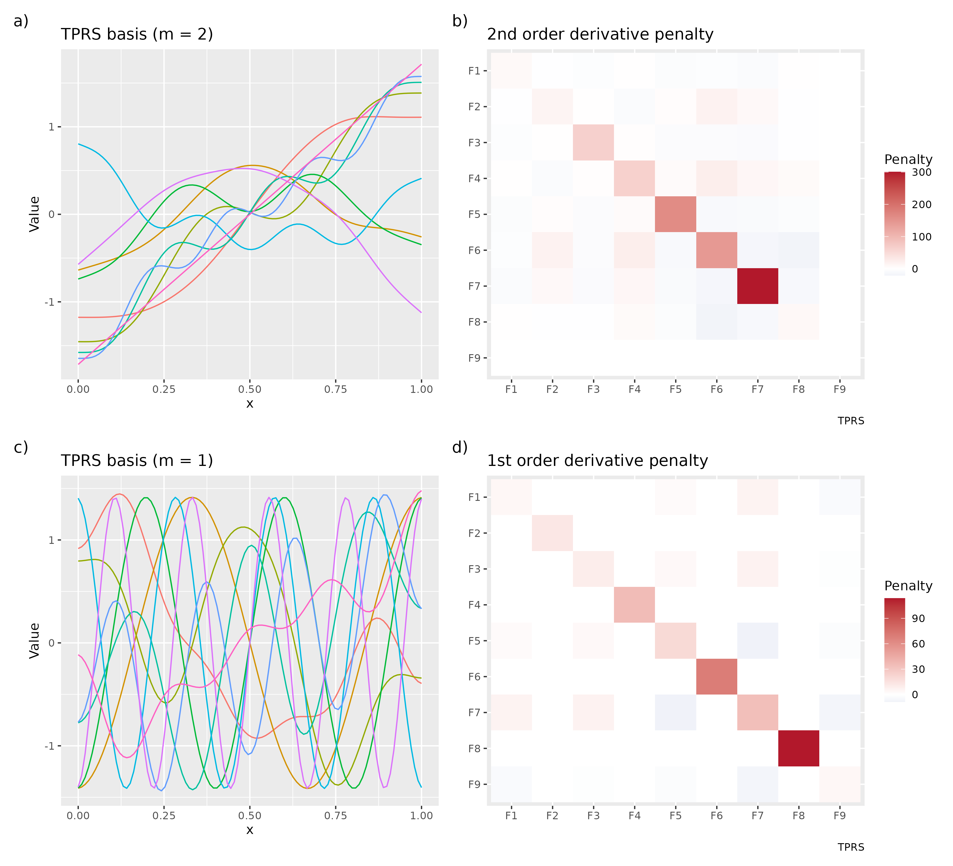
The figure below illustrates what is happening when you use m = 2 and m = 1 with the low-rank thin plate regression splines that are the default in mgcv's smooths.

The code to reproduce this is given at the end of this Answer, but do note that you'll need version >= 0.8.9.4 of gratia (which is not on CRAN, so follow instructions at the package homepage to install it).

The first row contains the default basis used in mgcv's smooths specified using s(): s(x, bs = "tp", m = 2, k = 10). The left panel (a) shows the basis functions, while the right panel (b) shows the penalty matrix $\mathbf{S}$ for this smooth. Note the linear basis function in the left panel (a). This function has 0 second derivative and as such it is not affected by the penalty. We say this function is in the penalty null space (and hence any linear function is in the penalty null space). This is reflected in the penalty matrix $\mathbf{S}$ shown in (b) as F9; the elements in the row/column relating to this function are 0.

When we switch to m = 1 with s(x, bs = "tp", m = 1, k = 10), we change the penalty to one based on the first derivative of the spline. This also changes the basis functions used for the smooth. The basis functions and penalty matrix $\mathbf{S}$ for this basis are shown in the lower row of the figure. There are still 9 basis functions (we lose 1 in both bases due to the identifiability constraint for the model constant term). The important difference is in the penalty matrix, where no functions except the constant function are in the penalty null space so we say this basis has no penalty null space (because we parameterise the constant term out of the basis with the identifiability constraint).

With the second order derivative penalty (m = 2) we are, as you rightly surmise, penalizing deviation from a linear function, where deviation is measured by the integrated squared second derivative of the estimated function. Because of the penalty null space, the simplest smooth we can produce with this basis and penalty is a linear function using 1 EDF. There are ways to penalize this even further, but this requires an explicit penalty on the null space, for example via select = TRUE in mgcv. When we use m = 1, we are penalizing deviation from a constant function (with deviation measured by the integrated squared first derivative of the estimated function). As the simplest function we can estimate using this basis and penalty combination is a flat constant function, degrees of freedom of the smooth can be penalized back to <1 EDF. With m = 1, a linear function would contribute to the penalty because the first derivative of any linear function that is not the constant function has a non-zero first derivative.

What difference does the choice of m make?

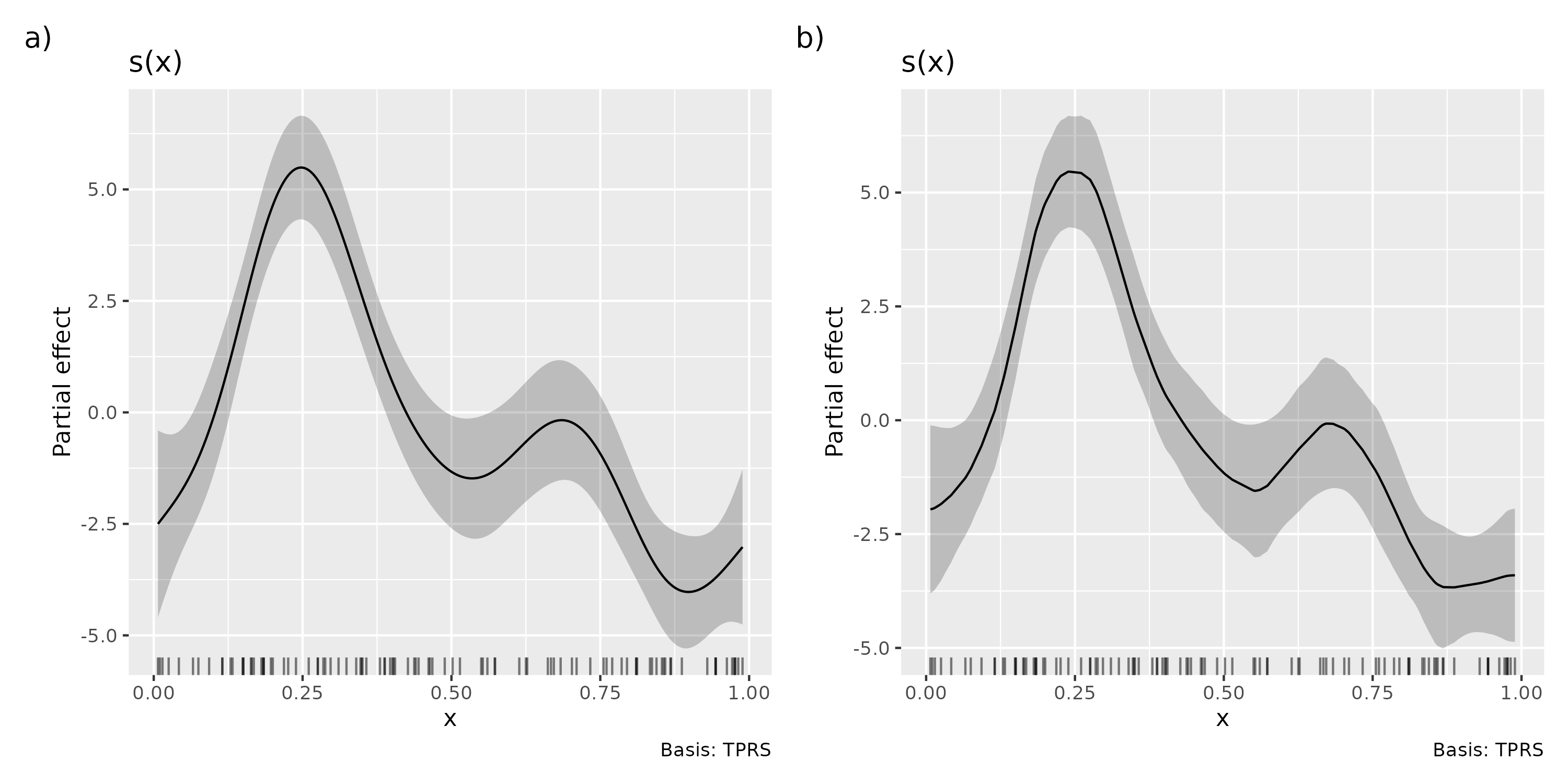
Consider this example, where data has been simulated from Gu and Wabha's $f_2$ function, that is smooth and non-linear

library("gratia")
library("mgcv")
library("patchwork")

df <- data_sim("gwf2", n = 100, seed = 2)

m_pen2 <- gam(y ~ s(x, m = 2, bs = "tp", k = 10), data = df, method = "REML")
m_pen1 <- gam(y ~ s(x, m = 1, bs = "tp", k = 10), data = df, method = "REML")

plt_a <- draw(m_pen2, n = 400)
plt_b <- draw(m_pen1, n = 400)

plt_a + plt_b +
  plot_layout(ncol = 2) +
  plot_annotation(tag_levels = "a", tag_suffix = ")")

Panel (a) is visually smoother than panel (b). Panel (a) uses the default m = 2 penalty, whereas the visually less-smooth fit in (b) was achieved by setting m = 1. The reason m = 2 is default is I suspect that in this branch of statistics, what has most often been considered as "smooth" are functions that are continuous up to second derivative because this is also what human see as being smooth — higher order derivatives such as the third which are not continuous aren't something that we typically notice. Cubic regression splines, for example, are important in this area, and those smooths meet this definition, and they are continuous up to second derivatives. That is not to say that other penalties/derivatives are not useful or needed. Indeed, they often are.

does it make sense to choose m=1 in cases where the edf is shrunk towards zero?

I'm not sure I follow; you would typically choose m = 1 befor fitting and it is only after fitting is complete can you ask how many EDF the estimated smooth uses. We don't use the EDF of the smooth during fitting, although it is related to the wiggliness of the smooth, which is what is being penalized during fitting. You should choose the penalty order that meets your assumptions about the relationship between the response $y$ and the covariate $x$ that you wish to capture via the smooth function $f(x)$. In many scientific settings, it would be implausible to think that the effect of a covariate on the response could be so jerky and abrupt as that shown in panel (b) above. In other settings, (b) could be entirely justifiable.

What would be the interpretation of the spline in such cases?

That a smooth uses fewer than 1 EDF is nothing special; you can even have non-linear functions that use fewer than 1 EDF. They'll typically be simple functions, close to quadratics say, but they can be estimated. Just focus on the estimated function itself — plot it to visualise the effect of $f(x)$ on the response. If it is an approximately constant function then that implies that the given the sample of data to hand that the effect of $x$ on the response is likely small and indistinguishable from "no effect" (a constant function).

Another area where it can make sense to change the order of the penalty is when interest is on other features of the estimated function; for example, identifying turning points in biodiversity time series are of interest because they give us some idea if the ecosystem is changing (for better or worse). This requires us to get a good estimate of the second derivative of the estimated smooth function and to do that we may need to use a penalty on a higher derivative (the 3rd derivative say) so that the thing we are interested in estimating is not the subject of the penalization directly.

Everything that I write above assumes that you have used a basis that is sufficiently large so as to either include the true but unknown function $f(x)$ or a close approximation to it. Checking that the basis dimension was sufficiently large to represent the true function is an important part of model diagnostics with GAMS. You could very easily estimate a flat approximately constant function where the true function is a sine wave over multiple cycles, for example, if you don't have enough basis functions in the basis to begin with.

library("gratia")
library("mgcv")
library("patchwork")

df <- data.frame(x = seq(0, 1, length = 100))
tprs_2 <- s(x, bs = "tp", m = 2, k = 10)
tprs_1 <- s(x, bs = "tp", m = 1, k = 10)
bs_2 <- basis(tprs_2, data = df, constraints = TRUE)
bs_1 <- basis(tprs_1, data = df, constraints = TRUE)

pen_2 <- penalty(tprs_2, data = df, constraints = TRUE)
pen_1 <- penalty(tprs_1, data = df, constraints = TRUE)

plt_2 <- bs_2 |> draw(title = "TPRS basis (m = 2)") +
  pen_2 |> draw(title = "2nd order derivative penalty") +
  plot_layout(ncol = 2, nrow = 1)
plt_1 <- bs_1 |> draw(title = "TPRS basis (m = 1)") +
  pen_1 |> draw(title = "1st order derivative penalty") +
  plot_layout(ncol = 2, nrow = 1)

plt_2 / plt_1 +
  plot_annotation(tag_levels = "a", tag_suffix = ")")