Hypothesis testing for detecting a (damped) sinusoidal signal in noise

Question

I have a signal in white noise that has the following form: \begin{equation} r[t_i] = A e^{-t_i/\tau} \sin{(\omega t_i + \phi)} + n[t_i] \end{equation}

I would like to test whether the signal (1st term) at a known frequency $\omega$ is present against the null-hypothesis of pure noise. I know for the noise term (Poissonian with $N>>1$) the standard deviation. $\phi$ and $\tau$ are unknown, however $\tau$ should be long compared to $t_\mathrm{max}$.

Is there a statistical test for this purpose? (If there are already implemented tests, Python is preferred but any language is fine)

I simulate a signal e.g. by

import numpy as np
import matplotlib.pyplot as plt

np.random.seed(123)

# Signal parameters
f   = 0.25 # Known
tau = 50   # Unknown
phi = 0    # Unknown
A   = 0.07 # Unknown A<1

# Signal modeling
t = np.arange(25)
s = A*np.sin(2*np.pi*f*t+phi)*np.exp(-t/tau)


# Noise parameters:
N   = 20e3 # Mean number of counts (known)
c   = 0.3  # Contrast (known)

# Noise modeling
cts = N *(c-2-2*c*s)/(c-2)
r = np.random.poisson(cts) 
plt.plot(r)
plt.title('signal with noise')
plt.show()

Answer 1

My intuition tells me:

1. build an optimal filter using e.g. a correlation with your expected signal r(t_i): see first example under https://docs.scipy.org/doc/scipy/reference/generated/scipy.signal.correlate.html
2. Run this filter over 1000 or more random noise signals, and observe the maxima of the correlation signals.
3. Then do it for your signal. If this maximum exceeds the 95% quantile of the observed maxima under the null hypothesis, then reject the null hypothesis with significance level 5%

For why this is sound see Rogers post which relates statistical signal processing and matched filters (optimal filters).

Answer 2

It may be possible to use Bayesian statistics here.

Let's set testing aside for a moment and instead focus on estimation. If we can construct a model and assess the estimates of $A$, maybe we can say something substantive about the decay term.

A simple model in Stan would be

data {
    int n;
    array[n] int r;
    vector[n] t;
    real c;
    real N;
    real f;
}
parameters {
    real<lower=0> inv_tau;
    real<lower=-1, upper = 1> phi_scaled;
    real<lower=0, upper=1> A;
}
transformed parameters {
    vector[n] s = A .* sin(2 * pi() * f * t +  pi() * phi_scaled) .* exp(-t * inv_tau);
    vector[n] cts = N .*(c-2-2*c*s)./(c-2);
}
model{
    A ~ uniform(0, 1);
    phi_scaled ~ uniform(-1, 1);
    inv_tau ~ cauchy(0, 1);

    r ~ poisson(cts);
}
generated quantities {
   real estimated_tau = 1.0 / inv_tau;
   real estimated_phu = pi() * phi;
   
}

Here, I am modelling scaled_phi to be on the interval $[-1, 1]$ and simply multiplying it by $\pi$ in the signal part. Additionally, I am modelling the inverse of $\tau$ rather than tau because I typically find that small parameters are often modelled more easily than large ones.

When I run the model, I get good diagnostics (note, you will need to install cmdstan and cmdstanpy if you want to replicate this).

import numpy as np
import cmdstanpy
import matplotlib.pyplot as plt
import arviz as az
def simulate_data():
    rng = np.random.RandomState(123)

    # Signal parameters
    f   = 0.25 # Known
    tau = 50   # Unknown
    phi = 0    # Unknown
    A   = 0.07 # Unknown A<1

    # Signal modeling
    t = np.arange(25)
    s = A*np.sin(2*np.pi*f*t+phi)*np.exp(-t/tau)


    # Noise parameters:
    N   = 20e3 # Mean number of counts (known)
    c   = 0.3  # Contrast (known)

    # Noise modeling
    cts = N *(c-2-2*c*s)/(c-2)
    r = rng.poisson(cts) 


    return t, r, cts


def fit_model(*args, **kwargs):
    t, r, cts = simulate_data()

    model = cmdstanpy.CmdStanModel(stan_file="signal.stan")

    data = dict(t=t.tolist(), r=r.tolist(), n=r.size, f = 0.25, N = 20000, c = 0.3)

    fit = model.sample(data, **kwargs)

    return fit

fit = fit_model()

print(fit.diagnose())

Checking sampler transitions treedepth.
Treedepth satisfactory for all transitions.

Checking sampler transitions for divergences.
No divergent transitions found.

Checking E-BFMI - sampler transitions HMC potential energy.
E-BFMI satisfactory.

Effective sample size satisfactory.

Split R-hat values satisfactory all parameters.

Processing complete, no problems detected.

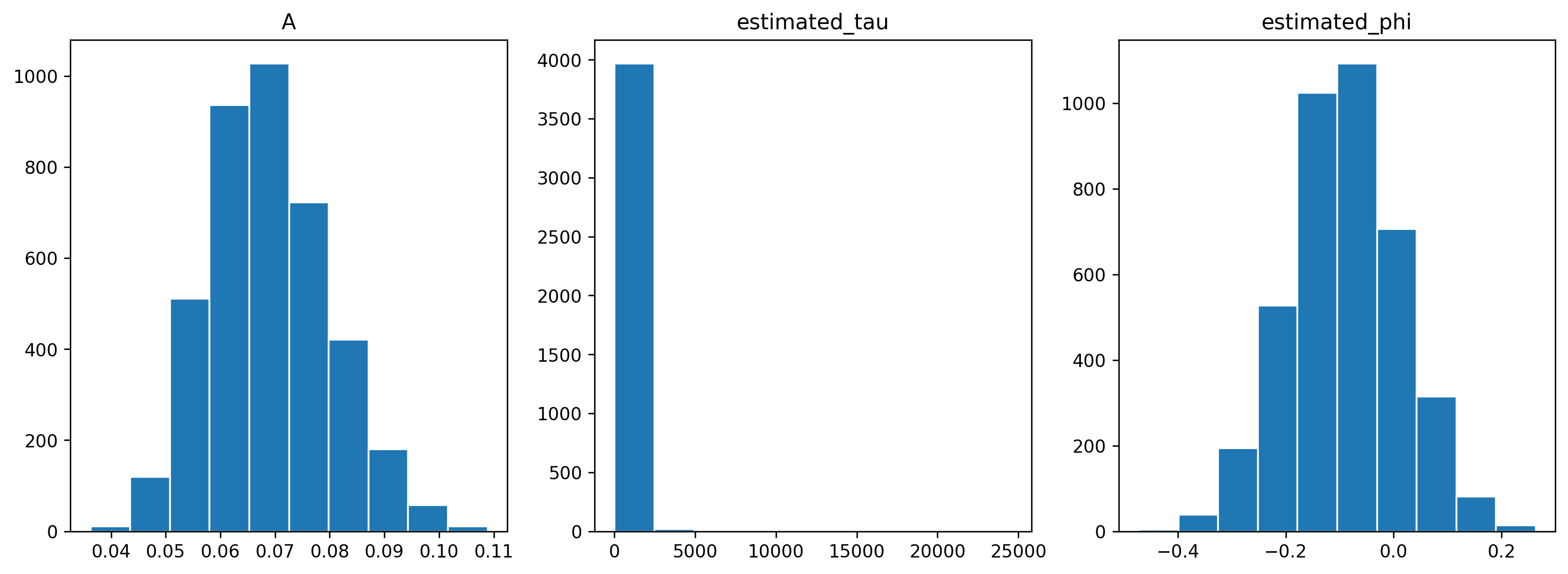
Now, we can look at some plots of the estimated parameters

var_names = ['A', 'estimated_tau', 'estimated_phi']

fig, ax = plt.subplots(dpi = 240, ncols=3, nrows=1, figsize = (15, 5))

for vn, a in zip(var_names, ax):
    x = fit.stan_variable(vn)
    a.hist(x, edgecolor='white')
    a.set_title(vn)

$A$ and $\phi$ are very well estimated. Tau remains uncertain (95% credible interval: 21 - 389), perhaps that could be combatted with some better priors.

From these plots, we could conclude that $A>0$ and hence the first term is likely present.

Answer 3

In engineering context likelihood ratio test is a typical approach for signal detection. The Poissonian noise for $N\gg 1$ can be viewed as Gaussian, which allows to write the joint probability density for the observations at the selected time moments $t_1,..., t_K$. This probability could be compared to the probability that the observations are purely due to the noise. One the compares the ratio of the two probabilities to a specified threshold to decide whether the signal is present or not.

The detailed derivations can be likely found in older (pre-digital era) radio-engineering or physics textbooks. After a bit of googling I found these notes on Statistical signal processing, which seem to be pretty close to what the OP is asking.