Can Survival Models model the time at which a random variable will first pass a certain point?

Question

Using standard survival models (e.g. Joint Survival Models), I could calculate the hazard and survival functions for individual cohorts at different time points in the future. Thus, I could make the naive argument that a standard Survival Model could show me when the average individual in a given cohort is expected to "pass a certain threshold for the first time".

Recently, I found out about First Passage Regression Models: https://www.jstatsoft.org/v66/i08/ . As I understand, these are based on the principles of Brownian Motions and explicitly model the first passage time.

To play devil's advocate - if I can do this with a Joint Survival Model, why do I need a First Passage Regression Model? What added advantages do I gain from a First Passage Regression Model instead of the standard Survival Model?

My guess is that using First Passage Regression Models (based on Brownian Motions), we end up with a full probability distribution of the first passage time instead of a point estimate - thus allowing for a richer analysis.

Is this interpretation correct?

Answer 1

As Cliff AB's answer noted, we need to distinguish between survival (a.k.a. time-to-event) data and specific models for that data (like Cox-PH, accelerated failure time, first passage models you mentioned and many others).

First consider a simple analogy: we have unbounded continous measurements and we are considering whether to model it with a normal, student-t or Gumbel distribution. The difference is that each makes different assumptions about the data.

Similarly, different models for time-to-event data make different assumptions about the underlying process. They also provide different interpretation of the data and analysis results. As any other model, they will perform well when their assumptions are met and poorly if they are grossly violated. Additionally, simpler/constrained models will tend to provide more precise estimates than complex/flexible models using the same amount of data.

To be specific, the first passage time model you mention is likely to be appealing if a convincing case can be made that there indeed is an underlying Wiener process. It will be particularly useful if we know the predictors act on the drift of the model, because this will provide a nice interpretation of model coefficients.

So e.g. modelling time to a stock hitting a value? Plausible. Time it takes a cell to complete a cell cycle? Maybe. Modelling a neurodegenerative disease? Unlikely as we know the underlying process is monotonous and thus not Wiener. More generally the independent increments assumption is going to be hard to justify for many real world processes as many processes have some form of momentum/memory/inner state.

The biggest possible advantage is that this model is quite restricted so if it is roughly correct, it will make good use of your data. The biggest disadvantage is that it is quite restricted and will thus be misleading/overconfident when a more flexible model is needed.

By contrast, Cox-PH model assumes that there is a fixed baseline hazard and any predictors act additively on the log-hazard. I don't think this has a very good direct physical interpretation, but the model is quite flexible and highly mathematically appealing and computationally tractable. It also naturally allows for predictors that change over time, multiple event types and other extensions that are hard to square with both first passage and accelerated failure time models.

It is true that the classical version of Cox-PH doesn't let you make direct predictions for time to event, but that can be ameliorated. One can restrict the class of baseline hazard functions to a semi-parametric form (e.g. a penalized spline for the log of baseline hazard) and then full predictions are possible. Indeed this is what Bayesian implementations of Cox-PH do.

One reason Cox-PH is often used is that the loss of power/precision due to its flexibility tends to be small for reasonably big datasets while the bias from an overly restricted model never goes away.

To some extent, you might be able to choose a good model based on data (e.g. via tests rejecting specific distributional forms, residual plots, comparing performance in cross-validation or posterior predictive check in the Bayesian context) but that will always be limited, so understanding how your data was collected and what it represents is crucial.

Answer 2

First threshold is not an alternative to survival analysis, but rather a distribution choice for survival analysis. To quote the abstract from the linked paper:

The threshold regression methodology is well suited to applications involving survival and time-to-event data, and serves as an important alternative to the Cox proportional hazards model.

The most popular survival regression model is the Cox-PH model, which involves a specific link function (proportional hazards) and a non-parametric baseline distribution. There is flexibility gained by using this non-parametric baseline, but the proportional hazards link may not always be appropriate.

Anecdotally, I find it very common that the proportional odds link is a better fit: the proportional hazards can have an outsized impact on the tails. Likewise, the accelerated failure time model with a Weibull baseline distribution is a common alternative to the Cox-PH model.

Answer 3

Cox proportional hazards models the probability/odds that an event is of type A or of type B, given that an event A or B happened. By doing that it avoids the problem of figuring out the probability of any hazard at all (whether it is A or B), and it only cares about the relative hazard.

So, that other package ignores this and models the events in some way by fitting a distribution for the passage times?

• The advantage of cox-ph is that you do not need to model the total hazard as function of time, and you only look at the relative hazards.
• The disadvantage of cox-ph is that you assume a specific model for the relative hazards (that it is independent of time) and that it contains all the information about the distributions.

If the absolute hazards, can be modeled, then I imagine that a model that does not ignore the absolute hazards might perform better.

---

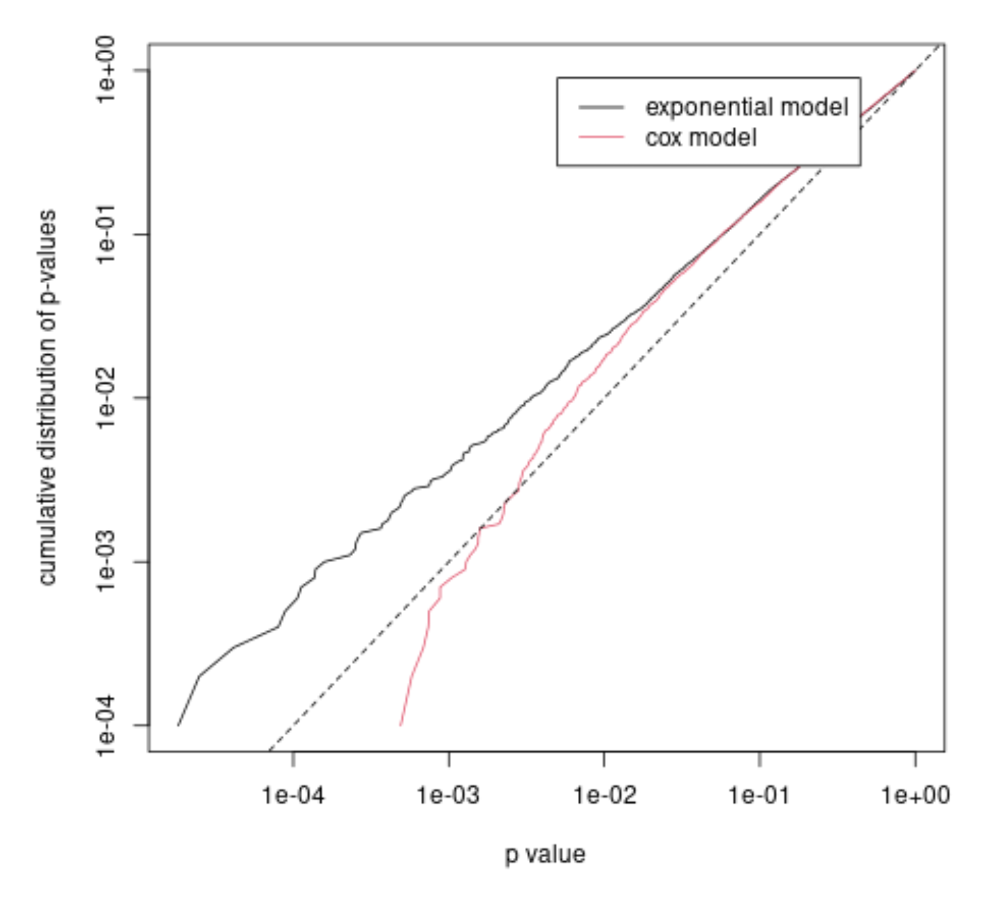
Below I simulate 1000 times an observation where there is an effect (so we expect a distribution of p-values that deviates from a uniform distribution, the stronger the deviation the higher the power). The cox model returns the low p-values less often than the exponential model (which models the passage times directly), and has less power.

^{The effect is very subtle and the difference is not so large. When I model with a glm model using a more general gamma distribution (the lines which have been commented out in the code below), instead of an exponential distribution, then the Cox model performs better and has larger power.}

library(survival)
set.seed(1)
n = 20
m = 10^4

pcox = rep(NA,m)
pexp = rep(NA,m)

### a function to
### - fit a nul model
### - fit an alternative model
### and compute p-value based on likelihood ratio
### assuming chi squared distribution for this value
pval_exp = function(time,x) {
    mu_0 = mean(time)
    mu_a = mean(time[x==0])
    mu_b = mean(time[x==1])
    lik_0 = sum(dexp(time,1/mu_0, log = 1))
    lik_1 = sum(dexp(time[x==0],1/mu_a, log = 1))+
            sum(dexp(time[x==1],1/mu_b, log = 1))
    D = 2*(lik_1-lik_0)
    return(1-pchisq(D,1))
}


### repeatedly simulate data with a non-zero-effect
### and compute p-values according to two models, one of them is Cox proportional hazerss
for (i in 1:m) {
  x = c(rep(1,n/2),rep(0,n/2))
  time = rexp(n,1+x*0.3)

  ##### the glm model below doesn't have great power
  ##### because it has a more flexible dispersion 
  ### mod = glm(time ~ x, family = Gamma(link = "identity"))
  ### pexp[i] = coef(summary(mod))[,4][2]

  ### the manual fitting with function pval_exp works better
  pexp[i] = pval_exp(time,x)

  mod2 = coxph(Surv(time) ~ x)
  pcox[i] = coef(summary(mod2))[5]
}

pexp = pexp[order(pexp)]
pcox = pcox[order(pcox)]

plot(pexp,c(1:m)/m, type = "l", ylab = "cumulative distribution of p-values", xlab = "p value", log = "xy")
lines(pcox,c(1:m)/m, col = 2)
lines(10^c(-10,1),10^c(-10,1), lty = 2, col = 1)

legend(0.005,0.9, c("exponential model", "cox model"), lty = 1, col = c(1,2) )

Answer 4

This might be naive, but : Accelerated Failure Time models model analyse the time to event. By encoding as 0 the individuals of the cohort which did not pass the threshold, and 1 the individuals which passed it at least once, you should be able to model the mean time to first passage of the threshold in each cohort?