"Can we believe the power values we compute?" Or "Do type I errors disappear as soon as the null is false"?

Question

This question was prompted by reading this short post: This is what “power=.06” looks like .
Seeing this brought back a question which has been nagging me, which I would describe as “Can we believe the power values we compute?”, or “Do type I errors disappear as soon as the null is false?”, or “Why is the power of our tests never lower that $\alpha$?"

When the null hypothesis is true, we observe type I errors ($\alpha$ errors, falsely rejecting the null, even though it is true). When the null is false, we have type II errors ($\beta$ errors, failing to reject the null when it is in fact false). Let’s take multiple 2-tailed 1-sample t-test (for simplicity). We sample from $N(0,.5)$ and test for a null of $\mu=0$. We will observe about $100\alpha$% significant results (false positives, type I errors). Let’s now repeat this, but now we sample from $N(0.01,.5)$ (or any other mean, which makes the power of the test very low). Technically, we can no longer have false positives (since the null is false). We will observe barely more than $100\alpha$% significant results; but in most of them, the effect will be grossly exaggerated, the observed mean will be very different from the true value. Our significant results will look very much like “false positives”. So did the type I errors really disappear, or are they in fact still there?

Let me call these exaggerated results False Significant (FS), by analogy with False Positives (FP). And let me define them as significant results, but where the CI of the statistic -here the mean- does not contain the true value of the statistic.
One could call them “type III” errors (e.g. see this CV post); but unfortunately, there is no agreed upon definition of type III errors. Mosteller defines them as “correctly rejecting the null for the wrong reason”, which is close but somehow broader. But Kaiser defines them as correctly rejecting the null, but in the wrong direction” (a narrower definition). And others define them as “errors committed by giving the right answer to the wrong problem” (which to me implies something different, e.g. like correctly testing the wrong null?). So, I will keep using FS, or False Significant, for this question.

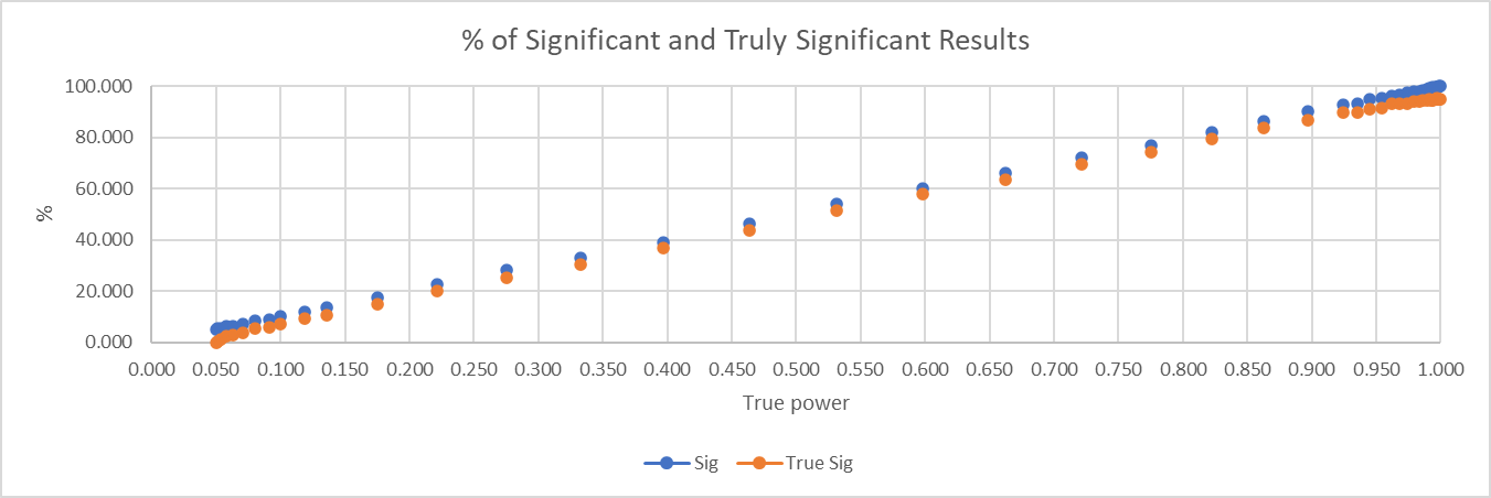
I then decided to run a quick simulation. 1-sample t, 20 random values drawn from N(0,.5) (no idea why I chose .5, but it would not matter anyway), $\alpha=.05$ (tradition), 10,000 iterations for each of several power levels, from .05 to .999 (done by changing the effect). For each10,000 test, I look at the proportion of significant results ($p<.05$), and of truly significant results ($p<.05$, and CI of mean contains the true mean), as a function of the true power (based on true effect, not observed one). I obtained the following graph;

It shows the proportion of significant results (blue), and truly significant results (orange). It is a bit hard to read, so I plotted the difference between the 2, i.e. the percentage (of all tests! Not just of the significant ones) which are FS. I obtained the following plot;

We can see that, in fact, the Type I errors do not disappear; they “morph” into FS. At very low power (close to .05), all the significant results are falsely significant. It is well known that for underpowered tests, most significant results have exaggerated effects; this simulation just further demonstrates this. Then, as the power increases, the false significant rate goes down, and stays steady for a good stretch (~ between power .2 and .8?) at around 2.5% (or really $\frac {\alpha} {2}$). And then increases again back to ~5% (really $\alpha$) as power gets close to .99. I can sort of intuitively understand why it starts by decreasing as the power increases, and why it plateaus at $\frac {\alpha} {2}$ (we can only get FS on one side anymore), but struggle with why it then increases back toward $\alpha$.

Now, finally (sorry for the long setup), to the questions;

1. Are these False Significant results really errors? (I think so). If so, they do not seem to get much attention; shouldn’t they?
2. Should we therefore discount the power values that we compute? (e.g. based on the simulation, for this test, a power of .06 is really a “true” power of ~.025)
3. Is there some intuitive explanation for the bathtub shape of the false significance? In particular, why does it grow again when we have very high power?
4. Should we give this phenomenon a name (we can agree on)? It is difficult to tackle an issue if it does not even have a (recognized) name.