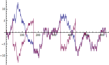
The correlation measures linear relationship. In informal context relationship means something stable. When we calculate the sample correlation for stationary variables and increase the number of available data points this sample correlation tends to true correlation.
It can be shown that for prices, which usually are random walks, the sample correlation tends to random variable. This means that no matter how much data we have, the result will always be different.
Note I tried expressing mathematical intuition without the mathematics. From mathematical point of view the explanation is very clear: Sample moments of stationary processes converge in probability to constants. Sample moments of random walks converge to integrals of brownian motion which are random variables. Since relationship is usually expressed as a number and not a random variable, the reason for not calculating the correlation for non-stationary variables becomes evident.
Update Since we are interested in correlation between two variables assume first that they come from stationary process $Z_t=(X_t,Y_t)$. Stationarity implies that $EZ_t$ and $cov(Z_t,Z_{t-h})$ do not depend on $t$. So correlation
$$corr(X_t,Y_t)=\frac{cov(X_t,Y_t)}{\sqrt{DX_tDY_t}}$$
also does not depend on $t$, since all the quantities in the formula come from matrix $cov(Z_t)$, which does not depend on $t$. So the calculation of sample correlation
$$\hat{\rho}=\frac{\frac{1}{T}\sum_{t=1}^T(X_t-\bar{X})(Y_t-\bar{Y})}{\sqrt{\frac{1}{T^2}\sum_{t=1}^T(X_t-\bar{X})^2\sum_{t=1}^T(Y_t-\bar{Y})^2}}$$
makes sense, since we may have reasonable hope that sample correlation will estimate $\rho=corr(X_t,Y_t)$. It turns out that this hope is not unfounded, since for stationary processes satisfying certain conditions we have that $\hat{\rho}\to\rho$, as $T\to\infty$ in probability. Furthermore $\sqrt{T}(\hat{\rho}-\rho)\to N(0,\sigma_{\rho}^2)$ in distribution, so we can test the hypotheses about $\rho$.
Now suppose that $Z_t$ is not stationary. Then $corr(X_t,Y_t)$ may depend on $t$. So when we observe a sample of size $T$ we potentialy need to estimate $T$ different correlations $\rho_t$. This is of course infeasible, so in best case scenario we only can estimate some functional of $\rho_t$ such as mean or variance. But the result may not have sensible interpretation.
Now let us examine what happens with correlation of probably most studied non-stationary process random walk. We call process $Z_t=(X_t,Y_t)$ a random walk if $Z_t=\sum_{s=1}^t(U_t,V_t)$, where $C_t=(U_t,V_t)$ is a stationary process. For simplicity assume that $EC_t=0$. Then
\begin{align}
corr(X_tY_t)=\frac{EX_tY_t}{\sqrt{DX_tDY_t}}=\frac{E\sum_{s=1}^tU_t\sum_{s=1}^tV_t}{\sqrt{D\sum_{s=1}^tU_tD\sum_{s=1}^tV_t}}
\end{align}
To simplify matters further, assume that $C_t=(U_t,V_t)$ is a white noise. This means that all correlations $E(C_tC_{t+h})$ are zero for $h>0$. Note that this does not restrict $corr(U_t,V_t)$ to zero.
Then
\begin{align}
corr(X_t,Y_t)=\frac{tEU_tV_t}{\sqrt{t^2DU_tDV_t}}=corr(U_0,V_0).
\end{align}
So far so good, though the process is not stationary, correlation makes sense, although we had to make same restrictive assumptions.
Now to see what happens to sample correlation we will need to use the following fact about random walks, called functional central limit theorem:
\begin{align}
\frac{1}{\sqrt{T}}Z_{[Ts]}=\frac{1}{\sqrt{T}}\sum_{t=1}^{[Ts]}C_t\to (cov(C_0))^{-1/2}W_s,
\end{align}
in distribution, where $s\in[0,1]$ and $W_s=(W_{1s},W_{2s})$ is bivariate Brownian motion (two-dimensional Wiener process). For convenience introduce definition $M_s=(M_{1s},M_{2s})=(cov(C_0))^{-1/2}W_s$.
Again for simplicity let us define sample correlation as
\begin{align}
\hat{\rho}=\frac{\frac{1}{T}\sum_{t=1}^TX_{t}Y_t}{\sqrt{\frac{1}{T}\sum_{t=1}^TX_t^2\frac{1}{T}\sum_{t=1}^TY_t^2}}
\end{align}
Let us start with the variances. We have
\begin{align}
E\frac{1}{T}\sum_{t=1}^TX_t^2=\frac{1}{T}E\sum_{t=1}^T\left(\sum_{s=1}^tU_t\right)^2=\frac{1}{T}\sum_{t=1}^Tt\sigma_U^2=\sigma_U\frac{T+1}{2}.
\end{align}
This goes to infinity as $T$ increases, so we hit the first problem, sample variance does not converge. On the other hand continuous mapping theorem in conjunction with functional central limit theorem gives us
\begin{align}
\frac{1}{T^2}\sum_{t=1}^TX_t^2=\sum_{t=1}^T\frac{1}{T}\left(\frac{1}{\sqrt{T}}\sum_{s=1}^tU_t\right)^2\to \int_0^1M_{1s}^2ds
\end{align}
where convergence is convergence in distribution, as $T\to \infty$.
Similarly we get
\begin{align}
\frac{1}{T^2}\sum_{t=1}^TY_t^2\to \int_0^1M_{2s}^2ds
\end{align}
and
\begin{align}
\frac{1}{T^2}\sum_{t=1}^TX_tY_t\to \int_0^1M_{1s}M_{2s}ds
\end{align}
So finally for sample correlation of our random walk we get
\begin{align}
\hat{\rho}\to \frac{\int_0^1M_{1s}M_{2s}ds}{\sqrt{\int_0^1M_{1s}^2ds\int_0^1M_{2s}^2ds}}
\end{align}
in distribution as $T\to \infty$.
So although correlation is well defined, sample correlation does not converge towards it, as in stationary process case. Instead it converges to a certain random variable.

