12
$\begingroup$

I am from an economics background and usually in the discipline the summary statistics of the variables are reported in a table. However, I wish to plot them.

I could modify a box plot to allow it to display the mean, standard deviation, minimum and maximum but I don't wish to do so as box plots are traditionally used to display medians and Q1 and Q3.

All of my variables have different scales. It would be great if somebody could suggest a meaningful way by which I could plot these summary statistics. I can work with R or Stata.

$\endgroup$
1
  • 1
    $\begingroup$ Welcome to the list. If you are asking about R commands then this question is off-topic here. But it seems you are asking primarily about what a good plot would look like and secondarily about how to create it. If so, I suggest deleting "with R" from your title and maybe stating, in the body, that you have R available. $\endgroup$
    – Peter Flom
    Commented Nov 27, 2013 at 11:38

2 Answers 2

17
$\begingroup$

There is a reason why Tukey's boxplot is universal, it can be applied to data derived from different distributions, from Gaussian to Poisson, etc. Median, MAD (median absolute deviation) or IQR (interquartile range) are more robust measures when data deviates from normality. However, mean and SD are more prone to outliers, and they should be interpreted with respect to the underlying distribution. The solution below is more suitable for normal or log-normal data. You may browse through a selection of robust measures here, and explore the WRS R package here.

# simulating dataset
set.seed(12)
d1 <- rnorm(100, sd=30)
d2 <- rnorm(100, sd=10)
d <- data.frame(value=c(d1,d2), condition=rep(c("A","B"),each=100))

# function to produce summary statistics (mean and +/- sd), as required for ggplot2
data_summary <- function(x) {
   mu <- mean(x)
   sigma1 <- mu-sd(x)
   sigma2 <- mu+sd(x)
   return(c(y=mu,ymin=sigma1,ymax=sigma2))
}

# require(ggplot2)
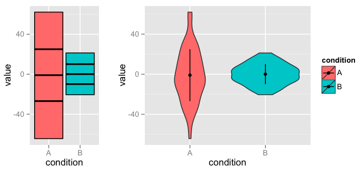
ggplot(data=d, aes(x=condition, y=value, fill=condition)) + 
geom_crossbar(stat="summary", fun.y=data_summary, fun.ymax=max, fun.ymin=min)

Additionally by adding + geom_jitter() or + geom_point() to the code above you can simultaneously visualise the raw data values.


Thanks to @Roland for pointing out the violin plot. It has an advantage in visualising probability density at the same time as summary statistic:

# require(ggplot2)
ggplot(data=d, aes(x=condition, y=value, fill=condition)) + 
geom_violin() + stat_summary(fun.data=data_summary)

Both examples are shown below.

enter image description here

$\endgroup$
9
  • 2
    $\begingroup$ I'd prefer a violin plot over this. $\endgroup$
    – Roland
    Commented Nov 27, 2013 at 15:42
  • 1
    $\begingroup$ Depending on the purpose of the analysis, mean and standard deviation is exactly what you need. I don't understand however the inconsistancy in R's summary.data.frame. It shows means but no sds. I can't think of many situations where means are useful but standard deviations misleading. $\endgroup$
    – Michael M
    Commented Nov 27, 2013 at 16:31
  • $\begingroup$ Indeed, sometimes you need to see the mean and the SD so that you judge whether they are useful.... $\endgroup$
    – Nick Cox
    Commented Nov 27, 2013 at 17:37
  • 1
    $\begingroup$ @TWL: The topic is much too broad to discuss here. But take for instance economic evaluations of drugs: For the patient, maybe it's important to know median treatment duration, while for the health insurance company it's the mean treatment duration because they need to pay it for each patient. A curious fact: In the case of the exponential distribution, mean +/- 1 standard deviation covers 68% of all mass, mean +/- 2 sds covers about 95% of all mass. As for the normal. (But it's mere chance ;)) $\endgroup$
    – Michael M
    Commented Nov 27, 2013 at 18:04
  • 1
    $\begingroup$ Thanks all, I like the proposed violin plots so will go ahead with that choice :-) $\endgroup$
    – Ridhima
    Commented Nov 28, 2013 at 15:11
9
$\begingroup$

There are myriad possibilities.

One option I have seen used which avoids confusion with boxplots (assuming you have medians or original data available) is to plot a boxplot and add a symbol that marks the mean (hopefully with a legend to make this explicit). This version of the boxplot that adds a marker for the mean is mentioned, for example in Frigge et al (1989) [1] :
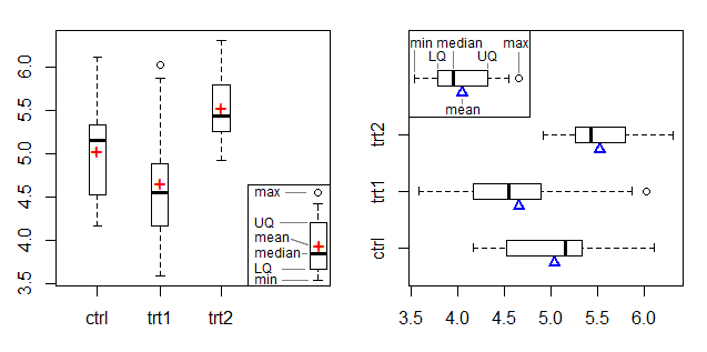
Boxplots showing mean marked as well

The left plot shows a + symbol as a mean marker and the right plot uses a triangle at the edge, adapting the mean marker from Doane & Tracy's beam-and-fulcrum plot [2].

See also this SO post and this one

If you don't have (or really don't want to show) the median a new plot will be needed and then it would be good for it to be visually distinct from a boxplot.

Perhaps something like this:
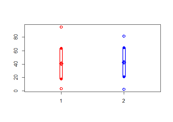
enter image description here

... which plots the minimum, maximum, mean and mean $\pm$ sd for each sample using different symbols and then draws a rectangle, or perhaps better, something like this:
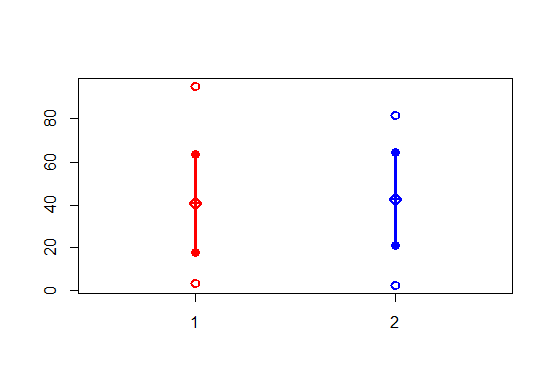
enter image description here

... which plots the minimum, maximum, mean and mean $\pm$ sd for each sample using different symbols and then draws a line (in fact at present that's actually a rectangle as before, but drawn narrow; it should be changed to drawing a line)

If your numbers are on very different scales, but are all positive, you might consider working with logs, or you might do small multiples with different (but clearly marked) scales

Code ( presently not particularly 'nice' code, but at the moment this is just exploring ideas, it's not a tutorial on writing good R code):

fivenum.ms=function(x) {r=range(x);m=mean(x);s=sd(x);c(r[1],m-s,m,m+s,r[2])}
eps=.015

plot(factor(c(1,2)),range(c(A,B)),type="n",border=0)
points((rep(c(1,2),each=5)),c(fivenum.ms(A),fivenum.ms(B)),col=rep(c(2,4),each=5),pch=rep(c(1,16,9,16,1),2),ylim=c(range(A,B)),cex=1.2,lwd=2,xlim=c(0.5,2.5),ylab="",xlab="")
rect(1-1.2*eps,fivenum.ms(A)[2],1+1.4*eps,fivenum.ms(A)[4],lwd=2,col=2,den=0)
rect(2-1.2*eps,fivenum.ms(B)[2],2+1.4*eps,fivenum.ms(B)[4],lwd=2,col=4,den=0)

plot(factor(c(1,2)),range(c(A,B)),type="n",border=0)
points((rep(c(1,2),each=5)),c(fivenum.ms(A),fivenum.ms(B)),col=rep(c(2,4),each=5),pch=rep(c(1,16,9,16,1),2),ylim=c(range(A,B)),cex=1.2,lwd=2,xlim=c(0.5,2.5),ylab="",xlab="")
rect(1-eps/9,fivenum.ms(A)[2],1+eps/3,fivenum.ms(A)[4],lwd=2,col=2,den=0)
rect(2-eps/9,fivenum.ms(B)[2],2+eps/3,fivenum.ms(B)[4],lwd=2,col=4,den=0)

[1] Frigge, M., D. C. Hoaglin, and B. Iglewicz (1989),
"Some implementations of the box plot."
American Statistician, 43 (Feb): 50-54.

[2] Doane D.P. and R.L. Tracy (2000),
"Using Beam and Fulcrum Displays to Explore Data"
American Statistician, 54(4):289–290, November

$\endgroup$

Your Answer

By clicking “Post Your Answer”, you agree to our terms of service and acknowledge you have read our privacy policy.

Not the answer you're looking for? Browse other questions tagged or ask your own question.