Determining whether the trend (or other component such as seasonality) is deterministic or stochastic is part of the puzzle in time series analysis. I will add a couple of points to what has been said.
1) The distinction between deterministic and stochastic trendsis important because if a unit root is present in the data (e.g. a random walk) then test statistics used for inference do not follow the traditional distribution. See this post for some details and references.
We can simulate a random walk (stochastic trend where first differences should be taken), test for the significance of deterministic trend and see the percentage of cases in which the null of deterministic trend is rejected. In R, we can do:
require(lmtest)
iter <- 10000
cval <- 0.05
n <- 120
rejections <- 0
set.seed(123)
for (i in seq.int(iter))
{
  x <- cumsum(rnorm(n)) # random walk
  fit <- lm(x ~ seq(n))
  if (coeftest(fit)[2,"Pr(>|t|)"] < cval)
    rejections <- rejections + 1
}
100 * rejections / iter
#[1] 88.67
At the 5% significance level, we would expect to reject the null in the 95% of cases, however, in this experiment it was rejected only in ~89% of cases out of 10,000 simulated random walks.
We can apply unit root tests to test whether a unit root is present. But we must be aware that a linear trend may in turn lead to failure to reject the null of a unit root. In order to deal with this, the KPSS test considers the null of stationarity around a linear trend.
2) Another issue is the interpretation of the deterministic components in a process in levels or first differences. The effect of an intercept is not the same in a model with a linear trend as in a random walk. See this post for illustration.
Analytically, let's take a random walk with drift:
$$
y_t = \mu + y_{t-1} + \epsilon_t \,,\quad \epsilon_t \sim NID(0, \sigma^2) \,.
$$
If we substitute repeatedly $y_{t-i}$ by lagged versions of $y_t$:
\begin{eqnarray*}
y_t &=& \mu + \underbrace{y_{t-1}}_{\mu + y_{t-2} + \epsilon_{t-1}} + \epsilon_t \\
&=& 2\mu + \underbrace{y_{t-2}}_{\mu + y_{t-3} + \epsilon_{t-2}} + \epsilon_{t-1} + \epsilon_t \\
&=& 3\mu + y_{t-3} + \epsilon_{t-2} + \epsilon_{t-1} + \epsilon_t \\
&...&
\end{eqnarray*}
We arrive to:
$$
y_t = y_0 + \mu t + \sum_{i=1}^t \epsilon_i
$$
where $y_0$ is some arbitrary initial value. Thus, we see that the accumulation of shocks and the long memory of the random walk makes the intercept $\mu$ to have the effect of a linear trend with slope $\mu$ (in this case the constant term $\mu$ is called a drift).
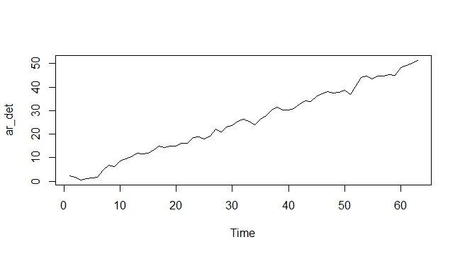
If the graphical representation of a series shows a relatively clear linear trend, we cannot be sure whether it is due to the presence of a deterministic linear trend or to a drift in a random walk process. Complementary graphics and tests statistics should be applied.
There are some caveats to bear in mind since an analysis based on unit root
and other test statistics is not foolproof. Some of these tests may be affected by the presence of outlying observations or level shifts and require the selection of a lag order which is not always straightforward.
As a workaround to this puzzle, I think that the common practice is to take differences of the data until the series looks stationary (for example looking at the autocorrelation function, which should go to zero fast) and then choose an ARMA model.


