Simplifying variable effects in a GLM in R

Question

Apologies, but it looks like my question is off topic for this forum. Thanks for all the excellent replies though. For those who have come across this question if they've been looking for something similar - then the short answer to my question below is very likely 'no'.

Please note this question has been edited in the light of the excellent responses below.

Can anyone recommend a way to easily ‘simplify’ the effects of variables in an R based GLM model? By simplify I mean any or all of the following:

• Group levels of a variable with similar effects.
• Apply a curve to the effects of an ordinal variable.
• Hand-smooth / alter the effects of a variable.
• Band (and re-band) a continuous variable.

Given that one has accepted the pros and cons of taking any of these approaches, are there any packages that might help with this? I’ve drawn a blank so far.

Thanks everyone for your responses.

For clarity (I hope) I have edited the question to remove the (inadvertent) confusing use of terminology , notably removing the use of ‘factor’, which I used in the original wording as a general term for ‘predictor variable’ rather than in the particular R sense of a variable with specific levels (something which as a relatively new user of R I unfortunately overlooked).

Also please note that I’m asking this question from an actuarial rather than a pure research standpoint.

In this field, there are reasonably well understood risk profiles (the chance of having a car accident, illness or death at different age for instance) and also a degree of leeway in applying ‘reasonable’ tweaks to the effects of individual variables (to the extent that most practitioners end up using software specifically designed for this purpose - a package called ‘Emblem’ being pretty much ubiquitous in the insurance industry in the UK).

I’m aware of the costs and benefits of treating any results in this way, but was just wondering if there were methods in R that could aid the process once the pros and cons are accepted.

Original Question:

Can anyone recommend a way to easily ‘simplify’ factors in an R based GLM model? By simplify I mean any or all of the following:

• Combine levels of a factor with similar effects.
• Apply a curve to the effects of a factor. Hand-smooth / alter the effects of a factor.
• Band (and re-band) factors in the model.

Are there any packages that might help with this? I’ve drawn a blank so far.

Answer 1

It's a simplification to have fewer parameters, but simplifying a model in the light of particular results has a cost too. Statistically-minded people differ in their views on modifying a model in the light of model results. Opposite arguments can both have merit: it's natural to want a model to be parsimonious as well as a good fit to the data (what else do we want?), but it's also risky to capitalise on chance and be over-responsive to what may be idiosyncrasies in a particular dataset. Some would argue that you are spending degrees of freedom in making such modifications; the question is whether the accountancy is honest and explicit. Whether there is a specific significance test that justifies a choice is not quite the issue here.

What is often neglected is the importance of fitting a model in a form that is both more transparent to the reader and easy for other researchers to compare given different data.

So consider this kind of statement:

"Factor $X$ as initially coded had 3 levels. But on an initial fit levels 2 and 3 were similar in their effects, so we merged them and the published model is for a two-level version."

(In some fields, you might be lucky to get this kind of explanation, as the project might be written up as if the final coding was that determined at the outset.)

There are at least two problems with this other than those already hinted at (discussed in various literatures under headings such as "data snooping"):

1. If it was thought worthwhile to use 3 levels in data production (e.g. these were the categories offered to people taking a questionnaire survey) there is information in the pattern of the coefficients, even if some seem similar in magnitude in one particular dataset.

2. This kind of adhockery makes it difficult for other researchers to do similar studies and check whether patterns are similar with other datasets. It's not obvious that the simplification defensible in one dataset will make sense with another dataset.

All of this implies, as a counsel of perfection, being open about initial and final models and why a model was modified. In practice there often need to be compromises and may be severe constraints depending on (e.g.) instructions from supervisors, conventions on reporting in different fields, or pressures from reviewers and editors on allowed space in journals.

This answer deliberately does not focus on what software might be used, within R or within any other statistical software, and why can now be explained. Model simplification does, and should, depend on substantive knowledge on what makes sense in the light of the underlying science, or in the light of practical knowledge about the situation in which the data were produced or in which the model is to be used. It is precisely the kind of decision that is, and should be, difficult to automate. That prejudice is, naturally, not a proof that software purporting to help is impossible or non-existent.

Answer 2

(@Nick Cox has done a good job talking about the issues involved in combining levels of a factor; I thought I would explain a little bit about categorical variables.)

It is not possible to 'fit a curve' to a categorical (nominal) variable. Nor is it possible to 'smooth' the fit. There are many ways to represent / code a factor (also here). Nonetheless, in one way or another, all methods use $k$ degrees of freedom to represent $k$ groups. In the end, the groups are fit by finding $k$ group means. By contrast, it is possible to have $k$ groups at fixed locations along a single, continuous variable (such as $0$ mg, $10$ mg, $20$ mg, etc.). In that case, a single degree of freedom can be expended to fit a straight line, or more for curved functions (e.g., $2$ for a curve with a single 'bend'). The implication of using $k$ degrees of freedom for $k$ groups is that each group is placed on its own dimension in the model's space. With, at most, $2$ groups on any dimension, curved functions are not meaningful. Thus, the reason you cannot find any R packages to do this is because it cannot be done. To illustrate, consider the following:

cont.x = c(1,1,1,1,1, 2,2,2,2,2, 3,3,3,3,3)
cat.x  = as.factor(c(1,1,1,1,1, 2,2,2,2,2, 3,3,3,3,3))
y      = c(1,2,3,4,5, 3,4,5,6,7, 5,6,7,8,9)

In both the continuous and categorical cases, what is entered is 1,2,3, but let's inspect the model matrices (a model matrix is how the variables are represented 'behind the scenes') and the resulting model fits:

model.matrix(lm(y~cont.x))
#    (Intercept) cont.x
# 1            1      1
# 2            1      1
# 3            1      1
# 4            1      1
# 5            1      1
# 6            1      2
# 7            1      2
# 8            1      2
# 9            1      2
# 10           1      2
# 11           1      3
# 12           1      3
# 13           1      3
# 14           1      3
# 15           1      3
# attr(,"assign")
# [1] 0 1
summary(lm(y~cont.x))
# ...
# Coefficients:
#             Estimate Std. Error t value Pr(>|t|)    
# (Intercept)   1.0000     1.0377   0.964  0.35282   
# cont.x        2.0000     0.4804   4.163  0.00111 **
#  ...

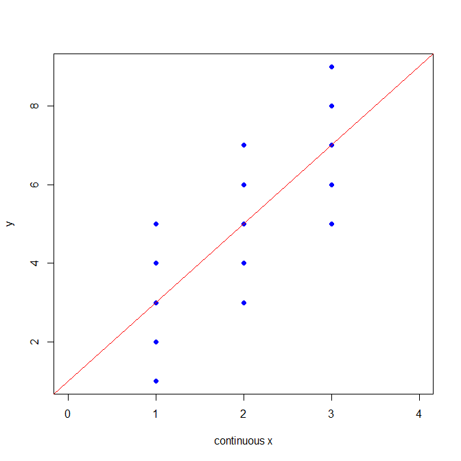
The continuous x is represented by a single variable. In the model fit, the slope of its line is given and the intercept is just the y value where the line crosses x=0. For the categorical x, it's different:

model.matrix(lm(y~cat.x))
#    (Intercept) cat.x2 cat.x3
# 1            1      0      0
# 2            1      0      0
# 3            1      0      0
# 4            1      0      0
# 5            1      0      0
# 6            1      1      0
# 7            1      1      0
# 8            1      1      0
# 9            1      1      0
# 10           1      1      0
# 11           1      0      1
# 12           1      0      1
# 13           1      0      1
# 14           1      0      1
# 15           1      0      1
# attr(,"assign")
# [1] 0 1 1
# attr(,"contrasts")
# attr(,"contrasts")$cat.x
# [1] "contr.treatment"
summary(lm(y~cat.x))
# ...
# Coefficients:
#             Estimate Std. Error t value Pr(>|t|)   
# (Intercept)   3.0000     0.7071   4.243  0.00114 **
# cat.x2        2.0000     1.0000   2.000  0.06866 . 
# cat.x3        4.0000     1.0000   4.000  0.00176 **
# ...

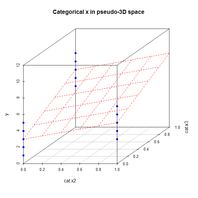
A separate variable is created for x=2 and for x=3, x=1 is indicated by 0's in both of those variables. In the model fit, the intercept now represents the mean of the first group, and the following two variables give the difference between the latter groups (each individually) and the first group.

Here are some pictures of what they look like: